Recent from talks
Nothing was collected or created yet.
Numerical analysis
View on Wikipedia

Numerical analysis is the study of algorithms that use numerical approximation (as opposed to symbolic manipulations) for the problems of mathematical analysis (as distinguished from discrete mathematics). It is the study of numerical methods that attempt to find approximate solutions of problems rather than the exact ones. Numerical analysis finds application in all fields of engineering and the physical sciences, and in the 21st century also the life and social sciences like economics, medicine, business and even the arts. Current growth in computing power has enabled the use of more complex numerical analysis, providing detailed and realistic mathematical models in science and engineering. Examples of numerical analysis include: ordinary differential equations as found in celestial mechanics (predicting the motions of planets, stars and galaxies), numerical linear algebra in data analysis,[2][3][4] and stochastic differential equations and Markov chains for simulating living cells in medicine and biology.
Before modern computers, numerical methods often relied on hand interpolation formulas, using data from large printed tables. Since the mid-20th century, computers calculate the required functions instead, but many of the same formulas continue to be used in software algorithms.[5]
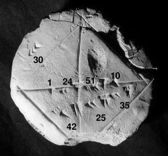
The numerical point of view goes back to the earliest mathematical writings. A tablet from the Yale Babylonian Collection (YBC 7289), gives a sexagesimal numerical approximation of the square root of 2, the length of the diagonal in a unit square.
Numerical analysis continues this long tradition: rather than giving exact symbolic answers translated into digits and applicable only to real-world measurements, approximate solutions within specified error bounds are used.
Applications
[edit]The overall goal of the field of numerical analysis is the design and analysis of techniques to give approximate but accurate solutions to a wide variety of hard problems, many of which are infeasible to solve symbolically:
- Advanced numerical methods are essential in making numerical weather prediction feasible.
- Computing the trajectory of a spacecraft requires the accurate numerical solution of a system of ordinary differential equations.
- Car companies can improve the crash safety of their vehicles by using computer simulations of car crashes. Such simulations essentially consist of solving partial differential equations numerically.
- In the financial field, (private investment funds) and other financial institutions use quantitative finance tools from numerical analysis to attempt to calculate the value of stocks and derivatives more precisely than other market participants.[6]
- Airlines use sophisticated optimization algorithms to decide ticket prices, airplane and crew assignments and fuel needs. Historically, such algorithms were developed within the overlapping field of operations research.
- Insurance companies use numerical programs for actuarial analysis.
History
[edit]The field of numerical analysis predates the invention of modern computers by many centuries. Linear interpolation was already in use more than 2000 years ago. Many great mathematicians of the past were preoccupied by numerical analysis,[5] as is obvious from the names of important algorithms like Newton's method, Lagrange interpolation polynomial, Gaussian elimination, or Euler's method. The origins of modern numerical analysis are often linked to a 1947 paper by John von Neumann and Herman Goldstine,[7][8] but others consider modern numerical analysis to go back to work by E. T. Whittaker in 1912.[7]

To facilitate computations by hand, large books were produced with formulas and tables of data such as interpolation points and function coefficients. Using these tables, often calculated out to 16 decimal places or more for some functions, one could look up values to plug into the formulas given and achieve very good numerical estimates of some functions. The canonical work in the field is the NIST publication edited by Abramowitz and Stegun, a 1000-plus page book of a very large number of commonly used formulas and functions and their values at many points. The function values are no longer very useful when a computer is available, but the large listing of formulas can still be very handy.
The mechanical calculator was also developed as a tool for hand computation. These calculators evolved into electronic computers in the 1940s, and it was then found that these computers were also useful for administrative purposes. But the invention of the computer also influenced the field of numerical analysis,[5] since now longer and more complicated calculations could be done.
The Leslie Fox Prize for Numerical Analysis was initiated in 1985 by the Institute of Mathematics and its Applications.
Key concepts
[edit]Direct and iterative methods
[edit]Direct methods compute the solution to a problem in a finite number of steps. These methods would give the precise answer if they were performed in infinite precision arithmetic. Examples include Gaussian elimination, the QR factorization method for solving systems of linear equations, and the simplex method of linear programming. In practice, finite precision is used and the result is an approximation of the true solution (assuming stability).
In contrast to direct methods, iterative methods are not expected to terminate in a finite number of steps, even if infinite precision were possible. Starting from an initial guess, iterative methods form successive approximations that converge to the exact solution only in the limit. A convergence test, often involving the residual, is specified in order to decide when a sufficiently accurate solution has (hopefully) been found. Even using infinite precision arithmetic these methods would not reach the solution within a finite number of steps (in general). Examples include Newton's method, the bisection method, and Jacobi iteration. In computational matrix algebra, iterative methods are generally needed for large problems.[9][10][11][12]
Iterative methods are more common than direct methods in numerical analysis. Some methods are direct in principle but are usually used as though they were not, e.g. GMRES and the conjugate gradient method. For these methods the number of steps needed to obtain the exact solution is so large that an approximation is accepted in the same manner as for an iterative method.
As an example, consider the problem of solving
- 3x3 + 4 = 28
for the unknown quantity x.
| 3x3 + 4 = 28. | |
| Subtract 4 | 3x3 = 24. |
| Divide by 3 | x3 = 8. |
| Take cube roots | x = 2. |
For the iterative method, apply the bisection method to f(x) = 3x3 − 24. The initial values are a = 0, b = 3, f(a) = −24, f(b) = 57.
| a | b | mid | f(mid) |
|---|---|---|---|
| 0 | 3 | 1.5 | −13.875 |
| 1.5 | 3 | 2.25 | 10.17... |
| 1.5 | 2.25 | 1.875 | −4.22... |
| 1.875 | 2.25 | 2.0625 | 2.32... |
From this table it can be concluded that the solution is between 1.875 and 2.0625. The algorithm might return any number in that range with an error less than 0.2.
Conditioning
[edit]Ill-conditioned problem: Take the function f(x) = 1/(x − 1). Note that f(1.1) = 10 and f(1.001) = 1000: a change in x of less than 0.1 turns into a change in f(x) of nearly 1000. Evaluating f(x) near x = 1 is an ill-conditioned problem.
Well-conditioned problem: By contrast, evaluating the same function f(x) = 1/(x − 1) near x = 10 is a well-conditioned problem. For instance, f(10) = 1/9 ≈ 0.111 and f(11) = 0.1: a modest change in x leads to a modest change in f(x).
Discretization
[edit]Furthermore, continuous problems must sometimes be replaced by a discrete problem whose solution is known to approximate that of the continuous problem; this process is called 'discretization'. For example, the solution of a differential equation is a function. This function must be represented by a finite amount of data, for instance by its value at a finite number of points at its domain, even though this domain is a continuum.
Generation and propagation of errors
[edit]The study of errors forms an important part of numerical analysis. There are several ways in which error can be introduced in the solution of the problem.
Round-off
[edit]Round-off errors arise because it is impossible to represent all real numbers exactly on a machine with finite memory (which is what all practical digital computers are).
Truncation and discretization error
[edit]Truncation errors are committed when an iterative method is terminated or a mathematical procedure is approximated and the approximate solution differs from the exact solution. Similarly, discretization induces a discretization error because the solution of the discrete problem does not coincide with the solution of the continuous problem. In the example above to compute the solution of , after ten iterations, the calculated root is roughly 1.99. Therefore, the truncation error is roughly 0.01.
Once an error is generated, it propagates through the calculation. For example, the operation + on a computer is inexact. A calculation of the type is even more inexact.
A truncation error is created when a mathematical procedure is approximated. To integrate a function exactly, an infinite sum of regions must be found, but numerically only a finite sum of regions can be found, and hence the approximation of the exact solution. Similarly, to differentiate a function, the differential element approaches zero, but numerically only a nonzero value of the differential element can be chosen.
Numerical stability and well-posed problems
[edit]An algorithm is called numerically stable if an error, whatever its cause, does not grow to be much larger during the calculation.[13] This happens if the problem is well-conditioned, meaning that the solution changes by only a small amount if the problem data are changed by a small amount.[13] To the contrary, if a problem is 'ill-conditioned', then any small error in the data will grow to be a large error.[13] Both the original problem and the algorithm used to solve that problem can be well-conditioned or ill-conditioned, and any combination is possible. So an algorithm that solves a well-conditioned problem may be either numerically stable or numerically unstable. An art of numerical analysis is to find a stable algorithm for solving a well-posed mathematical problem.
Areas of study
[edit]The field of numerical analysis includes many sub-disciplines. Some of the major ones are:
Computing values of functions
[edit]|
Interpolation: Observing that the temperature varies from 20 degrees Celsius at 1:00 to 14 degrees at 3:00, a linear interpolation of this data would conclude that it was 17 degrees at 2:00 and 18.5 degrees at 1:30pm. Extrapolation: If the gross domestic product of a country has been growing an average of 5% per year and was 100 billion last year, it might be extrapolated that it will be 105 billion this year. Regression: In linear regression, given n points, a line is computed that passes as close as possible to those n points. Optimization: Suppose lemonade is sold at a lemonade stand, at $1.00 per glass, that 197 glasses of lemonade can be sold per day, and that for each increase of $0.01, one less glass of lemonade will be sold per day. If $1.485 could be charged, profit would be maximized, but due to the constraint of having to charge a whole-cent amount, charging $1.48 or $1.49 per glass will both yield the maximum income of $220.52 per day. ![]() Differential equation: If 100 fans are set up to blow air from one end of the room to the other and then a feather is dropped into the wind, what happens? The feather will follow the air currents, which may be very complex. One approximation is to measure the speed at which the air is blowing near the feather every second, and advance the simulated feather as if it were moving in a straight line at that same speed for one second, before measuring the wind speed again. This is called the Euler method for solving an ordinary differential equation. |
One of the simplest problems is the evaluation of a function at a given point. The most straightforward approach, of just plugging in the number in the formula is sometimes not very efficient. For polynomials, a better approach is using the Horner scheme, since it reduces the necessary number of multiplications and additions. Generally, it is important to estimate and control round-off errors arising from the use of floating-point arithmetic.
Interpolation, extrapolation, and regression
[edit]Interpolation solves the following problem: given the value of some unknown function at a number of points, what value does that function have at some other point between the given points?
Extrapolation is very similar to interpolation, except that now the value of the unknown function at a point which is outside the given points must be found.[14]
Regression is also similar, but it takes into account that the data are imprecise. Given some points, and a measurement of the value of some function at these points (with an error), the unknown function can be found. The least squares-method is one way to achieve this.
Solving equations and systems of equations
[edit]Another fundamental problem is computing the solution of some given equation. Two cases are commonly distinguished, depending on whether the equation is linear or not. For instance, the equation is linear while is not.
Much effort has been put in the development of methods for solving systems of linear equations. Standard direct methods, i.e., methods that use some matrix decomposition are Gaussian elimination, LU decomposition, Cholesky decomposition for symmetric (or hermitian) and positive-definite matrix, and QR decomposition for non-square matrices. Iterative methods such as the Jacobi method, Gauss–Seidel method, successive over-relaxation and conjugate gradient method[15] are usually preferred for large systems. General iterative methods can be developed using a matrix splitting.
Root-finding algorithms are used to solve nonlinear equations (they are so named since a root of a function is an argument for which the function yields zero). If the function is differentiable and the derivative is known, then Newton's method is a popular choice.[16][17] Linearization is another technique for solving nonlinear equations.
Solving eigenvalue or singular value problems
[edit]Several important problems can be phrased in terms of eigenvalue decompositions or singular value decompositions. For instance, the spectral image compression algorithm[18] is based on the singular value decomposition. The corresponding tool in statistics is called principal component analysis.
Optimization
[edit]Optimization problems ask for the point at which a given function is maximized (or minimized). Often, the point also has to satisfy some constraints.
The field of optimization is further split in several subfields, depending on the form of the objective function and the constraint. For instance, linear programming deals with the case that both the objective function and the constraints are linear. A famous method in linear programming is the simplex method.
The method of Lagrange multipliers can be used to reduce optimization problems with constraints to unconstrained optimization problems.
Evaluating integrals
[edit]Numerical integration, in some instances also known as numerical quadrature, asks for the value of a definite integral.[19] Popular methods use one of the Newton–Cotes formulas (like the midpoint rule or Simpson's rule) or Gaussian quadrature.[20] These methods rely on a "divide and conquer" strategy, whereby an integral on a relatively large set is broken down into integrals on smaller sets. In higher dimensions, where these methods become prohibitively expensive in terms of computational effort, one may use Monte Carlo or quasi-Monte Carlo methods (see Monte Carlo integration[21]), or, in modestly large dimensions, the method of sparse grids.
Differential equations
[edit]Numerical analysis is also concerned with computing (in an approximate way) the solution of differential equations, both ordinary differential equations and partial differential equations.[22]
Partial differential equations are solved by first discretizing the equation, bringing it into a finite-dimensional subspace.[23] This can be done by a finite element method,[24][25][26] a finite difference method,[27] or (particularly in engineering) a finite volume method.[28] The theoretical justification of these methods often involves theorems from functional analysis. This reduces the problem to the solution of an algebraic equation.
Software
[edit]Since the late twentieth century, most algorithms are implemented in a variety of programming languages. The Netlib repository contains various collections of software routines for numerical problems, mostly in Fortran and C. Commercial products implementing many different numerical algorithms include the IMSL and NAG libraries; a free-software alternative is the GNU Scientific Library.
Over the years the Royal Statistical Society published numerous algorithms in its Applied Statistics (code for these "AS" functions is here); ACM similarly, in its Transactions on Mathematical Software ("TOMS" code is here). The Naval Surface Warfare Center several times published its Library of Mathematics Subroutines (code here).
There are several popular numerical computing applications such as MATLAB,[29][30][31] TK Solver, S-PLUS, and IDL[32] as well as free and open-source alternatives such as FreeMat, Scilab,[33][34] GNU Octave (similar to Matlab), and IT++ (a C++ library). There are also programming languages such as R[35] (similar to S-PLUS), Julia,[36] and Python with libraries such as NumPy, SciPy[37][38][39] and SymPy. Performance varies widely: while vector and matrix operations are usually fast, scalar loops may vary in speed by more than an order of magnitude.[40][41]
Many computer algebra systems such as Mathematica also benefit from the availability of arbitrary-precision arithmetic which can provide more accurate results.[42][43][44][45]
Also, any spreadsheet software can be used to solve simple problems relating to numerical analysis. Excel, for example, has hundreds of available functions, including for matrices, which may be used in conjunction with its built in "solver".
See also
[edit]- Category:Numerical analysts
- Analysis of algorithms
- Approximation theory
- Computational science
- Computational physics
- Gordon Bell Prize
- Interval arithmetic
- List of numerical analysis topics
- Local linearization method
- Numerical differentiation
- Numerical Recipes
- Probabilistic numerics
- Symbolic-numeric computation
- Validated numerics
Notes
[edit]References
[edit]Citations
[edit]- ^ "Photograph, illustration, and description of the root(2) tablet from the Yale Babylonian Collection". Archived from the original on 13 August 2012. Retrieved 2 October 2006.
- ^ Demmel, J.W. (1997). Applied numerical linear algebra. SIAM. doi:10.1137/1.9781611971446. ISBN 978-1-61197-144-6.
- ^ Ciarlet, P.G.; Miara, B.; Thomas, J.M. (1989). Introduction to numerical linear algebra and optimization. Cambridge University Press. ISBN 9780521327886. OCLC 877155729.
- ^ Trefethen, Lloyd; Bau III, David (1997). Numerical Linear Algebra. SIAM. ISBN 978-0-89871-361-9.
- ^ a b c Brezinski, C.; Wuytack, L. (2012). Numerical analysis: Historical developments in the 20th century. Elsevier. ISBN 978-0-444-59858-5.
- ^ Stephen Blyth. "An Introduction to Quantitative Finance". 2013. page VII.
- ^ a b Watson, G.A. (2010). "The history and development of numerical analysis in Scotland: a personal perspective" (PDF). The Birth of Numerical Analysis. World Scientific. pp. 161–177. ISBN 9789814469456.
- ^ Bultheel, Adhemar; Cools, Ronald, eds. (2010). The Birth of Numerical Analysis. Vol. 10. World Scientific. ISBN 978-981-283-625-0.
- ^ Saad, Y. (2003). Iterative methods for sparse linear systems. SIAM. ISBN 978-0-89871-534-7.
- ^ Hageman, L.A.; Young, D.M. (2012). Applied iterative methods (2nd ed.). Courier Corporation. ISBN 978-0-8284-0312-2.
- ^ Traub, J.F. (1982). Iterative methods for the solution of equations (2nd ed.). American Mathematical Society. ISBN 978-0-8284-0312-2.
- ^ Greenbaum, A. (1997). Iterative methods for solving linear systems. SIAM. ISBN 978-0-89871-396-1.
- ^ a b c Higham 2002
- ^ Brezinski, C.; Zaglia, M.R. (2013). Extrapolation methods: theory and practice. Elsevier. ISBN 978-0-08-050622-7.
- ^ Hestenes, Magnus R.; Stiefel, Eduard (December 1952). "Methods of Conjugate Gradients for Solving Linear Systems" (PDF). Journal of Research of the National Bureau of Standards. 49 (6): 409–. doi:10.6028/jres.049.044.
- ^ Ezquerro Fernández, J.A.; Hernández Verón, M.Á. (2017). Newton's method: An updated approach of Kantorovich's theory. Birkhäuser. ISBN 978-3-319-55976-6.
- ^ Deuflhard, Peter (2006). Newton Methods for Nonlinear Problems. Affine Invariance and Adaptive Algorithms. Computational Mathematics. Vol. 35 (2nd ed.). Springer. ISBN 978-3-540-21099-3.
- ^ Ogden, C.J.; Huff, T. (1997). "The Singular Value Decomposition and Its Applications in Image Compression" (PDF). Math 45. College of the Redwoods. Archived from the original (PDF) on 25 September 2006.
- ^ Davis, P.J.; Rabinowitz, P. (2007). Methods of numerical integration. Courier Corporation. ISBN 978-0-486-45339-2.
- ^ Weisstein, Eric W. "Gaussian Quadrature". MathWorld.
- ^ Geweke, John (1996). "15. Monte carlo simulation and numerical integration". Handbook of Computational Economics. Vol. 1. Elsevier. pp. 731–800. doi:10.1016/S1574-0021(96)01017-9. ISBN 9780444898579.
- ^ Iserles, A. (2009). A first course in the numerical analysis of differential equations (2nd ed.). Cambridge University Press. ISBN 978-0-521-73490-5.
- ^ Ames, W.F. (2014). Numerical methods for partial differential equations (3rd ed.). Academic Press. ISBN 978-0-08-057130-0.
- ^ Johnson, C. (2012). Numerical solution of partial differential equations by the finite element method. Courier Corporation. ISBN 978-0-486-46900-3.
- ^ Brenner, S.; Scott, R. (2013). The mathematical theory of finite element methods (2nd ed.). Springer. ISBN 978-1-4757-3658-8.
- ^ Strang, G.; Fix, G.J. (2018) [1973]. An analysis of the finite element method (2nd ed.). Wellesley-Cambridge Press. ISBN 9780980232783. OCLC 1145780513.
- ^ Strikwerda, J.C. (2004). Finite difference schemes and partial differential equations (2nd ed.). SIAM. ISBN 978-0-89871-793-8.
- ^ LeVeque, Randall (2002). Finite Volume Methods for Hyperbolic Problems. Cambridge University Press. ISBN 978-1-139-43418-8.
- ^ Quarteroni, A.; Saleri, F.; Gervasio, P. (2014). Scientific computing with MATLAB and Octave (4th ed.). Springer. ISBN 978-3-642-45367-0.
- ^ Gander, W.; Hrebicek, J., eds. (2011). Solving problems in scientific computing using Maple and Matlab®. Springer. ISBN 978-3-642-18873-2.
- ^ Barnes, B.; Fulford, G.R. (2011). Mathematical modelling with case studies: a differential equations approach using Maple and MATLAB (2nd ed.). CRC Press. ISBN 978-1-4200-8350-7. OCLC 1058138488.
- ^ Gumley, L.E. (2001). Practical IDL programming. Elsevier. ISBN 978-0-08-051444-4.
- ^ Bunks, C.; Chancelier, J.P.; Delebecque, F.; Goursat, M.; Nikoukhah, R.; Steer, S. (2012). Engineering and scientific computing with Scilab. Springer. ISBN 978-1-4612-7204-5.
- ^ Thanki, R.M.; Kothari, A.M. (2019). Digital image processing using SCILAB. Springer. ISBN 978-3-319-89533-8.
- ^ Ihaka, R.; Gentleman, R. (1996). "R: a language for data analysis and graphics" (PDF). Journal of Computational and Graphical Statistics. 5 (3): 299–314. doi:10.1080/10618600.1996.10474713. S2CID 60206680.
- ^ Bezanson, Jeff; Edelman, Alan; Karpinski, Stefan; Shah, Viral B. (1 January 2017). "Julia: A Fresh Approach to Numerical Computing". SIAM Review. 59 (1): 65–98. arXiv:1411.1607. doi:10.1137/141000671. hdl:1721.1/110125. ISSN 0036-1445. S2CID 13026838.
- ^ Jones, E., Oliphant, T., & Peterson, P. (2001). SciPy: Open source scientific tools for Python.
- ^ Bressert, E. (2012). SciPy and NumPy: an overview for developers. O'Reilly. ISBN 9781306810395.
- ^ Blanco-Silva, F.J. (2013). Learning SciPy for numerical and scientific computing. Packt. ISBN 9781782161639.
- ^ Speed comparison of various number crunching packages Archived 5 October 2006 at the Wayback Machine
- ^ Comparison of mathematical programs for data analysis Archived 18 May 2016 at the Portuguese Web Archive Stefan Steinhaus, ScientificWeb.com
- ^ Maeder, R.E. (1997). Programming in mathematica (3rd ed.). Addison-Wesley. ISBN 9780201854497. OCLC 1311056676.
- ^ Wolfram, Stephen (1999). The MATHEMATICA® book, version 4. Cambridge University Press. ISBN 9781579550042.
- ^ Shaw, W.T.; Tigg, J. (1993). Applied Mathematica: getting started, getting it done (PDF). Addison-Wesley. ISBN 978-0-201-54217-2. OCLC 28149048.
- ^ Marasco, A.; Romano, A. (2001). Scientific Computing with Mathematica: Mathematical Problems for Ordinary Differential Equations. Springer. ISBN 978-0-8176-4205-1.
Sources
[edit]- Golub, Gene H.; Charles F. Van Loan (1986). Matrix Computations (3rd ed.). Johns Hopkins University Press. ISBN 0-8018-5413-X.
- Ralston Anthony; Rabinowitz Philips (2001). A First Course in Numerical Analysis (2nd ed.). Dover publications. ISBN 978-0486414546.
- Higham, Nicholas J. (2002) [1996]. Accuracy and Stability of Numerical Algorithms. Society for Industrial and Applied Mathematics. ISBN 0-89871-355-2.
- Hildebrand, F. B. (1974). Introduction to Numerical Analysis (2nd ed.). McGraw-Hill. ISBN 0-07-028761-9.
- David Kincaid and Ward Cheney: Numerical Analysis : Mathematics of Scientific Computing, 3rd Ed., AMS, ISBN 978-0-8218-4788-6 (2002).
- Leader, Jeffery J. (2004). Numerical Analysis and Scientific Computation. Addison Wesley. ISBN 0-201-73499-0.
- Wilkinson, J.H. (1988) [1965]. The Algebraic Eigenvalue Problem. Clarendon Press. ISBN 978-0-19-853418-1.
- Kahan, W. (1972). A survey of error-analysis. Proc. IFIP Congress 71 in Ljubljana. Info. Processing 71. Vol. 2. North-Holland. pp. 1214–39. ISBN 978-0-7204-2063-0. OCLC 25116949. (examples of the importance of accurate arithmetic).
- Trefethen, Lloyd N. (2008). "IV.21 Numerical analysis" (PDF). In Leader, I.; Gowers, T.; Barrow-Green, J. (eds.). Princeton Companion of Mathematics. Princeton University Press. pp. 604–614. ISBN 978-0-691-11880-2.
External links
[edit]Journals
[edit]- Numerische Mathematik, volumes 1–..., Springer, 1959–
- volumes 1–66, 1959–1994 (searchable; pages are images). (in English and German)
- Journal on Numerical Analysis (SINUM), volumes 1–..., SIAM, 1964–
Online texts
[edit]- "Numerical analysis", Encyclopedia of Mathematics, EMS Press, 2001 [1994]
- Numerical Recipes, William H. Press (free, downloadable previous editions)
- First Steps in Numerical Analysis (archived), R.J.Hosking, S.Joe, D.C.Joyce, and J.C.Turner
- CSEP (Computational Science Education Project), U.S. Department of Energy (archived 2017-08-01)
- Numerical Methods, ch 3. in the Digital Library of Mathematical Functions
- Numerical Interpolation, Differentiation and Integration, ch 25. in the Handbook of Mathematical Functions (Abramowitz and Stegun)
- Tobin A. Driscoll and Richard J. Braun: Fundamentals of Numerical Computation (free online version)
Online course material
[edit]- Numerical Methods (Archived 28 July 2009 at the Wayback Machine), Stuart Dalziel University of Cambridge
- Lectures on Numerical Analysis, Dennis Deturck and Herbert S. Wilf University of Pennsylvania
- Numerical methods, John D. Fenton University of Karlsruhe
- Numerical Methods for Physicists, Anthony O’Hare Oxford University
- Lectures in Numerical Analysis (archived), R. Radok Mahidol University
- Introduction to Numerical Analysis for Engineering, Henrik Schmidt Massachusetts Institute of Technology
- Numerical Analysis for Engineering, D. W. Harder University of Waterloo
- Introduction to Numerical Analysis, Doron Levy University of Maryland
- Numerical Analysis - Numerical Methods (archived), John H. Mathews California State University Fullerton
Numerical analysis
View on GrokipediaHistory
Early foundations
The origins of numerical analysis trace back to ancient civilizations, where manual techniques were developed to approximate solutions to practical problems in geometry, astronomy, and engineering. In ancient Babylon, around 1800 BCE, mathematicians employed iterative methods to compute square roots, as evidenced by the clay tablet YBC 7289, which records an approximation of √2 as 1;24,51,10 in sexagesimal notation, accurate to about six decimal places. This approach, akin to the modern Babylonian method (also known as the Heronian method), involved successive approximations using the formula x_{n+1} = (x_n + a/x_n)/2, where a is the number under the root, demonstrating early recognition of convergence in iterative processes.[7][8] In ancient Greece, around 250 BCE, Archimedes advanced approximation techniques through the method of exhaustion, a precursor to integral calculus, to bound the value of π. By inscribing and circumscribing regular polygons with up to 96 sides within a circle of diameter 1, Archimedes established that 3 10/71 < π < 3 1/7, providing bounds accurate to about three decimal places and laying foundational principles for limit-based approximations in numerical geometry.[9][10] During the Renaissance, numerical methods gained momentum with tools for efficient computation. In 1614, John Napier introduced logarithms in his work Mirifici Logarithmorum Canonis Descriptio, defining them as a continuous product scaled to powers of a base close to 1 (specifically, 10^7), which transformed multiplication and division into addition and subtraction, revolutionizing astronomical and navigational calculations. Building on this, William Oughtred invented the slide rule in 1622, a mechanical analog device using two logarithmic scales that slide relative to each other to perform multiplication and division by aligning indices and reading products directly, as described in his Clavis Mathematicae.[11][12][13] Key 17th- and 18th-century contributions from prominent mathematicians further solidified interpolation and summation techniques essential to numerical analysis. Isaac Newton developed finite difference interpolation in the 1670s, as outlined in his unpublished manuscripts and later correspondence, using divided differences to construct polynomials that pass through given data points, enabling accurate estimation of intermediate values from discrete observations. Similarly, Leonhard Euler formulated summation rules in the 1730s, including the Euler-Maclaurin formula, which relates sums to integrals via Bernoulli numbers and derivatives, as presented in his Institutiones Calculi Differentialis (1755), providing a bridge between discrete and continuous mathematics for approximating series.[14][15][16][17] In the 19th century, efforts toward mechanization highlighted numerical analysis's practical applications. Charles Babbage proposed the Difference Engine in 1822, a mechanical device designed to automate the computation and tabulation of polynomial values using the method of finite differences, as detailed in his paper to the Royal Astronomical Society, aiming to eliminate human error in logarithmic and trigonometric tables. Accompanying Babbage's later Analytical Engine, Ada Lovelace's 1843 notes included a detailed algorithm for computing Bernoulli numbers up to the 7th order, written in a tabular format that specified operations like addition and looping, marking an early conceptual program for a general-purpose machine.[18][19][20][21] A notable example of 19th-century innovation is Horner's method for efficient polynomial evaluation, published by William George Horner in 1819 in his paper "A new method of solving numerical equations of all orders, by continuous approximation" to the Royal Society. This synthetic division technique reduces the number of multiplications required to evaluate a polynomial p(x) = a_n x^n + ... + a_1 x + a_0 at a point x_0 by nesting the computation as b_n = a_n, b_{k} = b_{k+1} x_0 + a_k for k = n-1 down to 0, with p(x_0) = b_0, avoiding the computational expense of explicit powers and minimizing round-off errors in manual calculations; it was particularly valuable for root-finding in higher-degree equations before electronic aids.[22][23]Development in the 20th century
The advent of electronic computing in the mid-20th century revolutionized numerical analysis, shifting it from manual and mechanical methods to automated processes capable of handling complex calculations at unprecedented speeds. The ENIAC, completed in 1945 by John Mauchly and J. Presper Eckert at the University of Pennsylvania, was designed specifically to compute artillery firing tables for the U.S. Army's Ballistic Research Laboratory, performing ballistic trajectory calculations that previously took hours by hand in mere seconds.[24][25] This machine's ability to solve systems of nonlinear differential equations numerically marked a pivotal step in applying computational power to real-world problems in physics and engineering, laying groundwork for modern numerical methods.[24] John von Neumann's contributions further propelled this evolution through his advocacy for the stored-program computer architecture, outlined in his 1945 EDVAC report, which separated computing from manual reconfiguration and enabled flexible execution of numerical algorithms.[26] This design influenced subsequent machines and emphasized the computer's role in iterative numerical computations, such as matrix inversions essential for scientific simulations.[27] Algorithmic advancements soon followed, with Gaussian elimination for solving linear systems gaining modern formalization in the 1940s through error analyses by Harold Hotelling and others, adapting the ancient method for electronic implementation and highlighting its stability in computational contexts.[28] Similarly, George Dantzig's simplex method, proposed in 1947, provided an efficient algorithm for linear programming problems, optimizing resource allocation in operations research and becoming a cornerstone for numerical optimization.[29][30] Error analysis emerged as a critical discipline amid these developments, with James H. Wilkinson's 1963 book Rounding Errors in Algebraic Processes offering the first comprehensive study of floating-point arithmetic errors in key computations like Gaussian elimination and eigenvalue calculations.[31] Wilkinson's backward error analysis framework demonstrated how rounding errors propagate in algebraic processes, establishing bounds that guide stable algorithm design and remain foundational in numerical software.[31] Alan Turing's 1948 report on the Automatic Computing Engine (ACE) also shaped numerical software by detailing a high-speed design for executing iterative methods, influencing early programming practices for scientific computing at the National Physical Laboratory.[32] Institutionally, the field grew rapidly post-World War II, driven by the need to apply mathematics to industry and defense. The Society for Industrial and Applied Mathematics (SIAM) was incorporated on April 30, 1952, to promote the development and application of mathematical methods, including numerical analysis, fostering collaboration among mathematicians, engineers, and scientists.[33] This era saw expanded post-war efforts in applied mathematics, with organizations like SIAM supporting conferences and research that integrated computing into numerical techniques, building on earlier international gatherings to address growing computational demands in the 1950s and 1960s.[34]Contemporary advancements
Since the 1990s, numerical analysis has increasingly incorporated parallel computing paradigms to address the demands of high-performance computing (HPC). The emergence of standardized parallel algorithms was marked by the release of the Message Passing Interface (MPI) standard in 1994, which provided a portable framework for message-passing in distributed-memory systems, enabling efficient scaling across multiprocessor architectures. This development facilitated the transition from sequential to parallel numerical methods, such as domain decomposition for solving partial differential equations on clusters. Exascale computing systems, capable of at least 10^18 floating-point operations per second (exaFLOPS), began widespread deployment in the early 2020s, starting with the U.S. Department of Energy's Frontier supercomputer achieving 1.1 exaFLOPS in 2022, followed by Aurora reaching 1.012 exaFLOPS in May 2024 and El Capitan achieving 1.742 exaFLOPS by November 2024, which as of November 2025 is the world's fastest supercomputer supporting advanced simulations in climate modeling and materials science.[35][36] In November 2025, a contract was signed for Alice Recoque, Europe's first exascale supercomputer based in France, powered by AMD and Eviden, further advancing international capabilities in AI, scientific computing, and energy-efficient research.[37] The integration of numerical analysis with machine learning has accelerated since the 2010s, particularly through neural networks employed as surrogate models to approximate complex computational processes. These models reduce the need for repeated evaluations of expensive numerical simulations, such as in optimization problems, by learning mappings from input parameters to outputs with high fidelity after training on limited data.[38] For uncertainty quantification, Bayesian methods have become prominent, treating numerical solutions as probabilistic inferences over posterior distributions to account for modeling errors and data variability in fields like fluid dynamics and structural analysis.[39] Notable events in the 2020s underscore the role of numerical advancements in crisis response, including DARPA high-performance computing initiatives, such as the 2010-launched Ubiquitous High-Performance Computing (UHPC) program, which evolved to influence energy-efficient architectures for exascale-era simulations amid broader 2020s efforts in resilient computing.[40] The COVID-19 pandemic in 2020 highlighted the impact of simulation-driven drug discovery, where physics-based numerical methods, combined with high-performance computing, accelerated virtual screening of molecular interactions to identify potential inhibitors for SARS-CoV-2 proteins, shortening traditional timelines from years to months.[41] Advances in stochastic methods have addressed big data challenges through variants of Monte Carlo techniques, exemplified by randomized singular value decomposition (SVD) algorithms introduced in the early 2010s, which provide low-rank approximations of large matrices with probabilistic guarantees, outperforming deterministic methods in speed for applications like principal component analysis on massive datasets.[42] The growth of open-source contributions has further democratized these tools, as seen in the evolution of the SciPy library since its inception in 2001, which has expanded to include robust implementations of parallel and stochastic numerical routines, fostering widespread adoption in scientific computing communities.[43]Fundamental Concepts
Classification of numerical methods
Numerical methods in numerical analysis are broadly classified into direct and iterative approaches based on how they compute solutions to mathematical problems. Direct methods produce an exact solution (within the limits of finite precision arithmetic) after a finite number of arithmetic operations, such as solving linear systems exactly via matrix factorizations.[44] In contrast, iterative methods generate a sequence of approximations that converge to the solution under suitable conditions, refining estimates step by step without guaranteeing an exact result in finite steps.[44] Another key distinction lies between deterministic and stochastic methods. Deterministic methods rely on fixed, repeatable procedures without incorporating randomness, ensuring the same output for identical inputs.[45] Stochastic methods, however, introduce randomness to handle uncertainty or complexity, such as in Monte Carlo integration for approximating high-dimensional integrals where traditional deterministic quadrature rules fail due to the curse of dimensionality.[46] Iterative methods can further be categorized by their formulation: fixed-point iterations reformulate the problem as finding a point where for some function , iterating until convergence; optimization-based methods, on the other hand, cast the problem as minimizing an objective function, using techniques like gradient descent to locate minima corresponding to solutions.[47] For instance, in root-finding, the bisection method operates directly by halving intervals containing a root, while the Newton-Raphson method iteratively approximates roots using local linearizations.[48] The efficiency of iterative methods is often assessed by their order of convergence, which quantifies how the error (where is the true solution) decreases with iterations. Linear convergence occurs when for a constant , reducing error proportionally each step; quadratic convergence holds when for some constant , squaring the error and accelerating near the solution. For example, bisection exhibits linear convergence with , halving the interval error per step, whereas Newton-Raphson achieves quadratic convergence under smoothness assumptions.[48] Convergence in iterative methods also depends on numerical stability, where small perturbations must not derail the process.[44]Discretization and approximation
Discretization in numerical analysis involves transforming continuous mathematical problems, such as differential equations defined over infinite domains, into discrete forms suitable for computation on finite grids or meshes. This process replaces continuous variables with discrete points or elements, enabling the use of algebraic equations to approximate solutions. Common techniques include grid-based methods like finite differences, which approximate derivatives using differences between function values at nearby grid points; spectral methods, which expand solutions in terms of global basis functions such as Fourier or Chebyshev polynomials for high accuracy in smooth problems; and finite element methods, which divide the domain into smaller elements and use local piecewise polynomials to represent the solution within each.[49][50][51] Approximation theory underpins these discretization techniques by providing mathematical frameworks for estimating continuous functions with simpler discrete representations. Taylor series offer a local approximation, expanding a function around a point using its derivatives to achieve high-order accuracy near that point, as formalized by Taylor's theorem. In contrast, global polynomial bases, such as Legendre or Chebyshev polynomials, approximate functions over the entire domain, leveraging properties like orthogonality for efficient computation and error control in methods like spectral approximations.[52][50] The order of approximation quantifies the accuracy of these methods, indicating how the error decreases with finer discretization. For instance, the central finite difference approximation for the first derivative is second-order accurate, given by where the error is proportional to , derived from the Taylor expansion of around .[52][50] A practical example of discretization arises in solving ordinary differential equations (ODEs), where the forward Euler method approximates the solution to with initial condition by using a first-order forward difference: with grid spacing determining the time step between discrete points . This method is simple but illustrates the core idea of replacing the continuous derivative with a discrete increment.[53] Mesh refinement, by reducing grid spacing or element size, improves approximation accuracy but incurs a trade-off with computational cost, as finer meshes increase the number of operations required, often scaling cubically in three dimensions for finite element methods.[49]Conditioning of problems
In numerical analysis, the conditioning of a problem quantifies its inherent sensitivity to small perturbations in the input data, determining how much such changes can amplify errors in the output. A well-conditioned problem exhibits limited sensitivity, allowing reliable computation even with imprecise inputs, whereas an ill-conditioned problem can lead to drastically different outputs from minor input variations, making accurate solutions challenging regardless of the computational method employed. This distinction is crucial for assessing the feasibility of numerical solutions before selecting algorithms. The foundational framework for evaluating problem conditioning stems from Jacques Hadamard's criteria for well-posedness, introduced in his 1902 lectures, which require that a problem possess a solution, that the solution be unique, and that the solution depend continuously on the input data (i.e., exhibit stability under small perturbations). Problems failing these criteria are deemed ill-posed; for instance, certain inverse problems in partial differential equations may lack existence or uniqueness, or their solutions may vary discontinuously with data changes. Hadamard's criteria emphasize that conditioning assesses the problem's intrinsic properties, not the solution method. For linear systems , where is an invertible matrix, the condition number provides a precise measure of conditioning, defined as using a consistent matrix norm such as the 2-norm or infinity-norm. This value acts as an amplification factor: the relative error in the computed solution satisfies , approximately bounding the output error by times the input perturbation for small errors. A condition number near 1 indicates excellent conditioning, while values exceeding or more signal severe ill-conditioning, often arising in applications like geophysical modeling. Illustrative examples highlight ill-conditioning's impact. In polynomial interpolation, the Vandermonde matrix with entries for distinct points becomes severely ill-conditioned as the points cluster or as the degree increases, with growing exponentially (e.g., for equispaced points in ), leading to unstable coefficient computations despite exact arithmetic. Similarly, the Hilbert matrix with entries exemplifies extreme ill-conditioning, where in the 2-norm, rendering even low-order systems (e.g., ) practically unsolvable due to sensitivity to rounding. These cases underscore how geometric or algebraic structures can inherently degrade conditioning. Backward error analysis complements conditioning by viewing computed solutions through a perturbation lens: a numerical algorithm produces that exactly solves a slightly perturbed problem , where the backward errors and are small relative to machine precision. This perspective, pioneered by Wilkinson, reveals that well-designed algorithms keep backward errors bounded independently of conditioning, but the forward error in still scales with , emphasizing the need to separate problem sensitivity from algorithmic reliability.[54] Notably, conditioning is an intrinsic property of the mathematical problem, independent of the algorithm chosen to solve it; however, poor conditioning necessitates careful algorithm selection, such as specialized solvers for stiff ordinary differential equation systems to mitigate amplification effects. This independence guides numerical analysts in prioritizing problem reformulation or regularization when is large.Error Analysis
Round-off errors
Round-off errors arise from the finite precision of computer arithmetic, where real numbers are approximated using a limited number of bits, leading to inaccuracies in representation and computation. In numerical analysis, these errors are inherent to floating-point systems and can significantly affect the reliability of algorithms, particularly when small perturbations propagate through operations.[55] The predominant standard for floating-point representation is IEEE 754, first established in 1985 and revised in 2008 to include enhancements like fused multiply-add operations and support for decimal formats, with a further minor revision in 2019 that provided clarifications, bug fixes, and additional features.[56][57] It defines binary formats such as single precision (32 bits, approximately 7 decimal digits) and double precision (64 bits, approximately 15-16 decimal digits), where numbers are stored as sign, exponent, and significand.[58] The machine epsilon, , represents the smallest relative difference between 1 and the next representable number greater than 1; for double precision, .[59] A fundamental bound on the representation error is given by where denotes the floating-point approximation of a real number .[60] This relative error ensures that well-scaled numbers are represented accurately to within a small fraction, but arithmetic operations like addition and multiplication introduce further round-off during evaluation. One major source of round-off error is subtractive cancellation, where subtracting two nearly equal numbers leads to a loss of significant digits. For instance, computing in double precision yields exactly 0 due to the loss of the small perturbation beyond the precision limit, exemplifying catastrophic cancellation. Such errors occur because the result has fewer significant bits than the inputs, amplifying relative inaccuracies.[55] In iterative processes like summation, round-off errors accumulate as low-order bits are discarded in each addition. The Kahan summation algorithm mitigates this by maintaining a compensation term to recover lost precision, reducing the total error bound from to nearly for terms. Developed in 1965, it is widely used in numerical libraries for more accurate accumulation.[61] The impact of round-off errors is particularly pronounced in ill-conditioned problems, where small input perturbations lead to large output variations, magnifying these precision limitations.[55]Truncation and discretization errors
Truncation error arises in numerical methods when an infinite process, such as a series expansion, is approximated by terminating it after a finite number of terms. A classic example occurs in the Taylor series expansion of a function around a point , where the approximation is used, and the truncation error is given by the remainder term for some between and .[62] This error quantifies the difference between the exact function value and its polynomial approximation, and its magnitude depends on the higher-order derivatives of and the distance from the expansion point.[63] Discretization error, closely related but distinct, emerges when continuous mathematical models are approximated on discrete grids or with finite steps, leading to inconsistencies between the numerical scheme and the underlying differential or integral equation. In the context of ordinary differential equations (ODEs), consistency of a method requires that the local truncation error—the error introduced in a single step assuming previous steps are exact—approaches zero as the step size tends to zero faster than . For Runge-Kutta methods, which approximate solutions to ODEs via weighted averages of function evaluations, the local truncation error is typically , where is the order of the method, ensuring consistency when .[64][65] A representative example of discretization error appears in numerical integration using the trapezoidal rule, which approximates over subintervals of width as . The global error for this method is for some , assuming is continuous, yielding an bound.[66] To derive this, consider a single interval ; the exact integral is for some and , while the trapezoidal approximation is , and applying Taylor expansions around reveals the local error per step, summing to globally over the interval.[67] To mitigate truncation and discretization errors, techniques like Richardson extrapolation combine approximations at different step sizes to eliminate leading error terms and achieve higher-order accuracy. For a method with error , computing and allows extrapolation to , effectively reducing the error order from to .[68] This approach is particularly effective for integration rules like the trapezoidal method, where repeated extrapolation yields Romberg integration with exponential convergence.[69] In consistent numerical methods, truncation and discretization errors converge to zero as the step size , enabling the approximate solution to approach the exact one, though this must be balanced against round-off errors that amplify with smaller .[70] The rate of convergence is determined by the order of the method, with higher-order schemes reducing these errors more rapidly for sufficiently smooth problems.[71]Error propagation and numerical stability
Error propagation in numerical computations refers to the way small initial errors, such as those from rounding or approximations, amplify or diminish as they pass through successive steps of an algorithm. Forward error analysis quantifies the difference between the exact solution and the computed solution, often expressed as the relative forward error , where is the exact solution and is the computed one.[72] In contrast, backward error analysis examines the perturbation to the input data that would make the computed solution exact for the perturbed problem, measured by the relative backward error , providing insight into an algorithm's robustness.[72] For linear systems , backward error is commonly assessed via the residual , where is the computed solution; a small indicates that solves a nearby system with small perturbations and .[73] Numerical stability ensures that errors do not grow uncontrollably during computation. An algorithm is backward stable if the computed solution is the exact solution to a slightly perturbed input problem, with perturbations bounded by machine epsilon times a modest function of the problem size.[73] For instance, the Householder QR decomposition is backward stable, producing factors and such that with , where is the unit roundoff, making it reliable for solving least squares problems.[73] In the context of finite difference methods for linear partial differential equations (PDEs), the Lax equivalence theorem states that a consistent scheme converges if and only if it is stable, where consistency means the local truncation error approaches zero as the grid spacing , and stability bounds the growth of solutions over time.[74] This theorem underscores that stability is essential for convergence in well-posed linear problems. A classic example of stability's impact is polynomial evaluation. The naive method of computing by successive powering and multiplication can lead to exponential error growth due to repeated squaring, whereas Horner's method, which rewrites the polynomial as , requires only multiplications and additions, achieving backward stability with a backward error bounded by .[75] Gaussian elimination without pivoting illustrates instability through the growth factor , where is the upper triangular factor; in the worst case, , causing severe error amplification in floating-point arithmetic.[76] For ordinary differential equation (ODE) solvers, A-stability requires the stability region to include the entire left half of the complex plane, ensuring bounded errors for stiff systems with eigenvalues having negative real parts. Dahlquist's criterion reveals that A-stable linear multistep methods have order at most 2, limiting explicit methods and favoring implicit ones like the trapezoidal rule for stiff problems.[77]Core Numerical Techniques
Computing function values
Computing function values in numerical analysis involves evaluating elementary and special functions using algorithms that ensure accuracy and efficiency, often leveraging series expansions, recurrences, and approximations to handle the limitations of finite-precision arithmetic.[78] For elementary functions like the exponential and trigonometric functions, Taylor series expansions provide a foundational method for numerical evaluation. The exponential function is approximated by its Taylor series , truncated at a suitable order based on the desired precision and the magnitude of , with convergence guaranteed for all real .[79] Similarly, the sine function uses , which converges rapidly for small and is computed term-by-term until the terms fall below the machine epsilon.[78] To extend these expansions to larger arguments, particularly for periodic functions like sine and cosine, argument reduction is essential: the input is reduced modulo to a primary interval such as , using high-precision representations of to minimize phase errors in floating-point arithmetic.[80] Special functions, such as Bessel functions, are often evaluated using recurrence relations for stability and efficiency. The Bessel function of the first kind satisfies the three-term recurrence , with initial values computed via series or asymptotic approximations; forward recurrence is stable for increasing when is fixed, allowing computation of higher-order values from lower ones.[81] For the gamma function , the Lanczos approximation offers a continued fraction representation that converges rapidly for , expressed as , where is a scaling parameter (often 5 or 7), are precomputed coefficients, and the error is bounded by machine precision for modest . This method, introduced by Lanczos in 1964, avoids the poles of the gamma function and is widely implemented in mathematical software libraries. Advanced algorithms for function approximation often employ Chebyshev polynomials to achieve minimax error, minimizing the maximum deviation over an interval. The Chebyshev polynomial of the first kind satisfies , and expansions in these polynomials provide near-optimal uniform approximations for continuous functions on , with the error equioscillating at points, closely matching the true minimax polynomial. For example, the constant can be computed using Machin-like formulas, which combine arctangent evaluations via identities such as ; each arctangent is approximated by its Taylor series for , converging quickly due to the small arguments.[82] To prevent overflow and underflow in computations involving logarithms and exponentials, scaling techniques are applied, such as rewriting as to keep exponents within representable ranges, or using specialized functions like for small to avoid catastrophic cancellation.[83] These strategies ensure numerical stability across a wide dynamic range in floating-point systems.Interpolation and regression
Interpolation in numerical analysis involves constructing a continuous function that exactly passes through a discrete set of given data points for , enabling estimation of the underlying function at intermediate points. This process is essential for approximating functions from tabular data, with polynomial interpolation being a primary approach where the interpolant is a polynomial of degree at most . Regression extends this by seeking an approximating function that minimizes the error across the data points, often using least squares to handle noisy or overdetermined systems. Both techniques rely on basis functions or divided differences for efficient computation, and function evaluation methods can be applied to compute basis values during construction.[84] Polynomial interpolation can be formulated using the Lagrange basis polynomials, defined as , where the interpolating polynomial is . This form, attributed to Joseph-Louis Lagrange, provides a direct expression for the unique polynomial of degree at most passing through the points, though it is computationally expensive for large due to the product evaluations.[85] Alternatively, Newton's divided difference interpolation offers a more efficient recursive structure, expressing as , where the divided differences are computed iteratively from the data values. This method, originating from Isaac Newton's work on finite differences, allows adding points incrementally and is numerically stable when points are ordered.[86] For smoother approximations, especially with unequally spaced data or to avoid oscillations, spline interpolation uses piecewise polynomials joined with continuity constraints. Cubic splines, consisting of cubic polynomials between knots with continuous first and second derivatives at the knots, provide smoothness and are widely used for their balance of flexibility and computational tractability. Carl de Boor's seminal work formalized the theory and algorithms for such splines, emphasizing their role in approximation. B-splines, a basis for representing splines, enhance stability by localizing support—each B-spline of degree influences only intervals—and facilitate stable numerical evaluation via de Boor's algorithm. De Boor's 1976 survey established B-splines as fundamental for spline computations, proving key representation theorems.[87] In regression, the goal shifts to fitting a model to data that may not lie exactly on a low-degree polynomial, typically by minimizing the squared residual sum , where is the design matrix and the observation vector. The solution satisfies the normal equations , first systematically derived by Adrien-Marie Legendre in 1805 for orbital computations and probabilistically justified by Carl Friedrich Gauss in his 1809 work Theoria Motus Corporum Coelestium.[88] This linear system can be ill-conditioned for high-degree polynomials or multicollinear features, leading to overfitting where the model captures noise rather than the signal. A classic illustration of interpolation challenges is the Runge phenomenon, observed by Carl Runge in 1901, where high-degree polynomial interpolation on equispaced points over for produces large oscillations near the endpoints, diverging as degree increases. This instability arises from the Lebesgue constant growth and can be mitigated by using Chebyshev nodes, clustered near endpoints, which bound the error more effectively for analytic functions.[89] To address overfitting in regression, regularization adds a penalty term, such as ridge regression's , shrinking coefficients to improve generalization on noisy data. Introduced by Hoerl and Kennard in 1970, this method stabilizes the normal equations by conditioning , reducing variance at the cost of slight bias.[90]Solving nonlinear equations
Solving nonlinear equations involves finding roots of functions where , a fundamental problem in numerical analysis applicable to scalar and multivariable cases. Iterative methods are typically employed due to the lack of closed-form solutions for most nonlinear problems, relying on initial approximations and successive refinements to achieve convergence to the root. These techniques must balance efficiency, robustness, and accuracy, often requiring analysis of convergence properties to ensure reliability.[91] For scalar nonlinear equations, the bisection method provides a reliable bracketing approach by repeatedly halving an interval known to contain a root, assuming the function changes sign at the endpoints per the intermediate value theorem. This method guarantees convergence but at a linear rate, making it slower than higher-order alternatives for well-behaved functions. The secant method, an extension of the false position method, approximates the derivative using two prior points to update the estimate via the formula achieving superlinear convergence without requiring derivative evaluations, though it may fail if points coincide or the function is ill-conditioned.[92][91] In multidimensional settings, Newton's method generalizes to systems of nonlinear equations by using the Jacobian matrix to solve for the update where , offering quadratic convergence near the root if the Jacobian is invertible and the initial guess is sufficiently close. This requires computing and inverting the Jacobian at each step, which can be computationally expensive for large systems.[93] Convergence of iterative root-finding methods is characterized by the order , where the error for some asymptotic constant , with indicating linear convergence and quadratic. Fixed-point iteration reformulates the problem as and iterates , converging linearly if at the fixed point . The contraction mapping theorem ensures unique fixed points and global linear convergence in complete metric spaces if is a contraction, i.e., there exists such that for all .[94][95] Nonlinear systems arise in applications like chemical equilibrium, where equations model reaction balances and require solving coupled nonlinearities for species concentrations. Quasi-Newton methods, such as Broyden's approach, approximate the Jacobian iteratively without full recomputation, updating via a rank-one modification to achieve superlinear convergence while reducing costs compared to full Newton steps. For instance, Broyden's method maintains an approximation satisfying secant conditions .[96][97] To promote global convergence, especially from distant initial guesses, safeguards like line search are incorporated into Newton-like methods, adjusting the step length along the search direction to satisfy descent conditions such as Armijo's rule, ensuring sufficient decrease in a merit function like . These techniques mitigate divergence risks in nonconvex problems while preserving local quadratic rates.[98]Linear Algebra Methods
Direct methods for linear systems
Direct methods for linear systems provide exact solutions to the equation in a finite number of arithmetic operations by factorizing the coefficient matrix into triangular forms that enable substitution. These algorithms are particularly suited for dense or structured matrices where the factorization cost is manageable, offering reliability when the matrix is well-conditioned.[99] The cornerstone of these methods is Gaussian elimination, which systematically eliminates variables below the diagonal to transform into an upper triangular matrix , while recording the elimination steps in a lower triangular matrix with unit diagonal entries, yielding the LU decomposition . This factorization, first formulated in modern matrix terms by Turing in his analysis of rounding errors, allows the system to be solved in two stages: forward substitution to solve for , followed by back substitution to solve . The forward substitution process computes for to , and back substitution computes , for down to .[100][99] To mitigate numerical instability from small pivots, partial pivoting is incorporated by interchanging rows at each elimination step to select the entry of largest magnitude in the current column below the pivot, which bounds the growth of elements during factorization and ensures backward stability in floating-point arithmetic. The growth factor, defined as the maximum absolute value in the transformed matrix divided by the maximum in , serves as a diagnostic for potential ill-conditioning; values close to 1 indicate robust computation, while large growth signals risks from the matrix's conditioning.[99][101] For symmetric positive definite matrices, the Cholesky decomposition exploits symmetry to factor , where is lower triangular with positive diagonal entries, requiring roughly half the operations of LU and avoiding pivoting since positive definiteness guarantees stable pivots. The algorithm computes the Cholesky factor column-by-column, with the -th column satisfying and for , originally developed by Cholesky for geodetic computations and published posthumously.[102][99] The computational complexity of LU or Cholesky factorization for a dense matrix is , dominated by the elimination phase, with forward and back substitution each requiring ; for multiple right-hand sides, the factorization is performed once and reused. Specialized variants exploit structure: for banded matrices with bandwidth , the cost reduces to , and for sparse matrices, fill-reducing orderings preserve sparsity to keep operations sub-cubic. In particular, tridiagonal systems () are solved via the Thomas algorithm, a direct LU variant that performs forward elimination without pivoting in time, computing modified diagonals and then substituting; it assumes diagonal dominance for stability and is widely used in finite difference methods for differential equations.[99] The reliability of these methods is closely tied to the conditioning of , as poorly conditioned matrices amplify errors despite stable factorization.[99]Iterative methods for linear systems
Iterative methods provide approximate solutions to large-scale linear systems , where is sparse and the system size precludes direct methods, by generating a sequence of iterates that converge to the exact solution under suitable conditions.[45] These methods are particularly effective for matrices arising from discretizations of partial differential equations, as they exploit sparsity to reduce computational cost and memory usage compared to exact factorizations.[45] Convergence acceleration techniques, such as preconditioning and multigrid, further enhance their efficiency for ill-conditioned problems.[45] Stationary iterative methods, which apply a fixed iteration matrix at each step, include the Jacobi and Gauss-Seidel methods. The Jacobi method updates each component independently using values from the previous iteration: for , assuming .[103] Developed by C.G.J. Jacobi in the 19th century, it decomposes , where is diagonal, strictly lower triangular, and strictly upper triangular, yielding the iteration .[104] The Gauss-Seidel method, introduced by P.L. von Seidel in 1874 building on earlier work by C.F. Gauss, updates components sequentially, incorporating newly computed values immediately, which corresponds to the iteration .[104] This forward substitution often leads to faster convergence than Jacobi for many matrices, though both require the iteration matrix to have spectral radius less than 1 for convergence.[103] Krylov subspace methods, which are non-stationary and generate iterates in increasingly larger subspaces, offer superior performance for large systems. The conjugate gradient (CG) method, proposed by M.R. Hestenes and E. Stiefel in 1952, is optimal for symmetric positive definite (SPD) matrices, minimizing the A-norm of the error over the Krylov subspace at each step.[105] For general nonsymmetric systems, the generalized minimal residual (GMRES) method, developed by Y. Saad and M.H. Schultz in 1986, minimizes the residual norm over the Krylov subspace, requiring restarts or truncation for practical implementation due to growing storage needs. Both methods converge in at most steps in exact arithmetic but typically require far fewer iterations when the effective dimension is low. Preconditioning transforms the system to or to improve conditioning, where has a smaller condition number than .[45] Simple diagonal preconditioning scales rows and columns by the reciprocals of diagonal entries, while incomplete LU (ILU) preconditioning approximates the LU factorization of by dropping small elements during elimination, as introduced by J.A. Meijerink and H.A. van der Vorst in 1977 for sparse matrices. For stationary methods, convergence requires the spectral radius of the preconditioned iteration matrix to be less than 1; for CG, the number of iterations to reduce the error by a factor of is bounded by .[105][103] A representative application is solving the discrete Poisson equation on a uniform grid, yielding a large sparse SPD system amenable to CG or multigrid acceleration. Multigrid methods, pioneered by A. Brandt in 1977, use coarse-grid corrections to eliminate low-frequency errors that stationary smoothers like Gauss-Seidel cannot resolve efficiently on fine grids.[106] By recursively restricting residuals to coarser levels, solving approximately, and prolongating corrections, multigrid achieves convergence independent of grid size in work for unknowns.[106] Iterative methods are well-suited for parallel computation on sparse systems, as matrix-vector products and local updates can be distributed across processors with minimal communication for structured grids or graph-based sparsity patterns.[45] This parallelism scales efficiently on modern architectures, making them essential for high-performance simulations.[45]Eigenvalue and singular value problems
Eigenvalue problems in numerical analysis concern the computation of scalars and nonzero vectors satisfying for a given square matrix , along with the related task of finding singular values and decompositions for rectangular matrices. These computations are fundamental for understanding matrix spectral properties, stability analysis, and dimensionality reduction in data. The power method provides an iterative approach to approximate the dominant eigenvalue (largest in magnitude) and its eigenvector, starting from an initial vector and updating via , which converges linearly under suitable conditions on the eigenvalue gap.[107] This method is simple and effective for matrices where one eigenvalue dominates, but it requires normalization at each step to prevent overflow and assumes the initial vector has a component in the dominant eigenspace.[107] For computing the full set of eigenvalues, the QR algorithm, developed by John G. F. Francis in the late 1950s, iteratively decomposes the matrix into an orthogonal and upper triangular such that , then sets , converging to a triangular form revealing the eigenvalues on the diagonal. Enhancements include deflation to isolate eigenvalues as they converge and Wilkinson shifts to accelerate convergence by targeting the bottom-right 2x2 submatrix, ensuring quadratic convergence for simple eigenvalues. The algorithm operates on matrices reduced to upper Hessenberg form (nonzero only on the main diagonal and subdiagonal, plus above), which preserves invariant subspaces and reduces computational cost while maintaining similarity to the original matrix.[108] Singular value decomposition (SVD) factorizes a matrix as , where and are orthogonal and is diagonal with nonnegative singular values , providing a generalization of eigendecomposition for non-square matrices. The Golub-Reinsch algorithm from 1970 first reduces to bidiagonal form using Householder transformations, then applies a variant of the QR algorithm to compute the singular values, achieving numerical stability and efficiency for dense matrices.[109] In applications, eigendecomposition underpins principal component analysis (PCA), where the covariance matrix's eigenvectors represent principal components that maximize variance in data projection, enabling dimensionality reduction while preserving key structure.[110] Standard dense eigenvalue algorithms, including QR-based methods, exhibit cubic computational complexity for an matrix, dominated by the orthogonal transformations.[107] For sparse matrices, iterative methods like the Lanczos algorithm (for symmetric matrices) and Arnoldi iteration (for general matrices) exploit structure by building Krylov subspaces through matrix-vector products, targeting extreme eigenvalues with lower cost per iteration, often per step but requiring many iterations.[107] These approaches leverage invariant subspaces for partial spectrum computation, avoiding full dense factorization.[111]Integration and Differentiation
Numerical quadrature
Numerical quadrature encompasses a variety of techniques for approximating the definite integral of a function, typically expressed as , where direct analytical evaluation is infeasible. These methods are essential in numerical analysis for applications ranging from physics simulations to financial computations, relying on discrete evaluations of the integrand to estimate the area under the curve. The choice of method depends on the function's properties, such as smoothness, dimensionality, and oscillatory behavior, with error bounds often derived from polynomial approximation theory.[112] Newton-Cotes formulas represent one foundational class of quadrature rules, derived by interpolating the integrand with polynomials over equidistant points and integrating the interpolant exactly. The simplest is the trapezoidal rule, which uses linear interpolation between endpoints to yield , with a global error of order for composite application over subintervals of width .[113] For higher accuracy, Simpson's rule employs quadratic interpolation over pairs of intervals, approximating the integral as for a single panel, achieving a composite error of order .[114] These rules are exact for polynomials up to the interpolation degree but suffer from Runge phenomenon for high-order variants on non-periodic functions.[115] Gaussian quadrature elevates precision by selecting optimal nodes and weights based on orthogonal polynomials, such as Legendre polynomials for the standard interval . An -point Gaussian rule is exact for all polynomials of degree at most , doubling the degree of exactness compared to Newton-Cotes for the same number of evaluations.[116] The nodes are the roots of the th orthogonal polynomial, and weights are computed via the Christoffel-Darboux formula or related methods, making it particularly efficient for smooth integrands.[112] To handle functions with varying smoothness, adaptive quadrature refines the mesh dynamically by estimating local errors and subdividing intervals where needed. A common error estimation technique involves step doubling: compute the integral over an interval using a coarse step and a refined step , then use the difference between these approximations as an error proxy, scaled by the method's order (e.g., factor of 15 for Simpson's rule).[117] If the estimated error exceeds a tolerance, the interval is recursively bisected until convergence, balancing computational cost with accuracy for non-uniform integrands like those with singularities.[118] In multidimensional settings, such as , deterministic methods like product Gauss rules face the curse of dimensionality, where the number of required evaluations grows exponentially as to maintain accuracy, rendering them impractical for .[119] Monte Carlo integration circumvents this by sampling points uniformly from the domain and estimating the integral as the expected value , with root-mean-square error scaling as independent of dimension.[120] Variance reduction techniques, such as importance sampling (reweighting samples toward regions of high variance) or stratified sampling (partitioning the domain into subregions), can further improve convergence without altering the dimensional independence.[121] For oscillatory integrals of the form or with , where causes rapid phase variations, standard rules like trapezoidal degrade due to cancellation errors. Filon's method addresses this by approximating the smooth amplitude with a low-degree polynomial (e.g., quadratic) at selected nodes and integrating exactly against the oscillatory factor, yielding an error of superior to for naive methods.[122] This approach, originally for trigonometric integrals, extends to more general phases via asymptotic analysis in modern variants.[123]Numerical differentiation
Numerical differentiation approximates the derivatives of a function using discrete samples, typically through finite difference methods that leverage Taylor series expansions to estimate rates of change. These techniques are essential in numerical analysis for scenarios where analytical derivatives are unavailable or impractical to compute directly. The simplest approaches include forward, backward, and central differences, each offering varying levels of accuracy based on the step size . The forward difference approximates the first derivative as , which has an error of order , while the backward difference uses with similar error characteristics. The central difference, , achieves higher accuracy with an error of , making it preferable for smooth functions.[124][125] To improve accuracy beyond second order, higher-order methods such as Richardson extrapolation combine multiple finite difference approximations at different step sizes to eliminate lower-order error terms. For instance, applying Richardson extrapolation to central differences at steps and yields an approximation of the first derivative, given by . This technique systematically refines estimates by assuming the error expansion is a power series in , allowing extrapolation to . It is particularly effective in applications requiring precise derivative estimates without increasing the stencil size excessively.[68][126] Automatic differentiation provides an alternative to finite differences by computing exact gradients through algorithmic differentiation of the function's computational graph, avoiding truncation errors entirely. In forward mode, derivatives propagate from inputs to outputs alongside the function evaluation, suitable for problems with few inputs and many outputs, with computational cost scaling linearly with the number of inputs. Reverse mode, conversely, computes gradients by backpropagating from outputs to inputs, efficient for scenarios with many inputs and few outputs, such as in optimization, and is foundational in machine learning frameworks. Both modes yield results accurate to machine precision, making them superior for differentiable programs.[127] Finite differences are commonly applied in the discretization of partial differential equations (PDEs), where they approximate spatial derivatives on a grid to convert continuous problems into solvable algebraic systems. For example, in solving the heat equation , central differences for the second derivative yield a stencil , enabling explicit or implicit time-stepping schemes. This approach underpins many finite difference methods for PDEs.[128] A key challenge in numerical differentiation arises with noisy data, where finite difference approximations amplify high-frequency noise, leading to unreliable derivative estimates. Differentiation acts as a high-pass filter, exacerbating errors proportional to , where is the noise standard deviation. To mitigate this, smoothing techniques such as splines are employed; cubic smoothing splines minimize a penalized least-squares objective, balancing data fit and smoothness to produce stable derivatives. These methods regularize the problem, reducing noise sensitivity while preserving underlying trends.[129][130] For noisy datasets, finite difference methods often underperform due to error amplification, prompting a preference for integration-based approaches that inherently smooth data and avoid direct derivative computation. This limitation underscores the need for hybrid strategies in practical applications involving experimental or observational data.[129]Differential Equations
Ordinary differential equations
Numerical methods for solving ordinary differential equations (ODEs) primarily address initial value problems of the form , , where is a vector in . These methods approximate the solution over a time interval by advancing from initial conditions using discrete steps of size . Explicit one-step methods, such as Runge-Kutta schemes, compute the next solution value directly from previous ones without solving additional equations, making them suitable for non-stiff problems where the solution varies smoothly.[131] Implicit methods, in contrast, require solving nonlinear equations at each step, offering superior stability for stiff systems where components evolve on vastly different timescales. Runge-Kutta methods form a cornerstone of explicit solvers, generalizing the Euler method by evaluating the right-hand side multiple times per step to achieve higher accuracy. The classical fourth-order Runge-Kutta (RK4) method, developed by Carl Runge in 1895 and refined by Martin Wilhelm Kutta in 1901, provides a local truncation error of and is widely used for its balance of simplicity and precision. Its implementation is specified via the Butcher tableau, a systematic representation introduced by John C. Butcher in 1963 that encodes the coefficients for stage evaluations and weighted combinations. For RK4, the tableau is:| 0 | |||
| 1/2 | 1/2 | ||
| 1/2 | 0 | 1/2 | |
| 1 | 0 | 0 | 1 |
| ----- | ----- | ----- | ----- |
| 1/6 | 1/3 | 1/3 |
Partial differential equations
Numerical methods for solving partial differential equations (PDEs) primarily address boundary value problems, where solutions are sought over spatial domains subject to specified conditions on the boundaries. These methods discretize the spatial derivatives to convert the PDE into a system of algebraic equations or ordinary differential equations (ODEs), enabling computational approximation. Key approaches include finite difference, finite element, and spectral methods, each suited to different problem characteristics such as domain geometry, boundary conditions, and solution smoothness. Finite volume methods, another key class, discretize the PDE by integrating over finite control volumes, ensuring local conservation of quantities like mass or momentum. They are particularly effective for hyperbolic PDEs and conservation laws, such as the Euler equations in fluid dynamics, by reconstructing fluxes at cell interfaces (e.g., using Godunov's method or higher-order schemes like MUSCL). This approach handles discontinuities like shocks robustly and is widely used in computational fluid dynamics.[132] Finite difference methods approximate derivatives using Taylor expansions on a structured grid, replacing continuous operators with discrete differences. For the Laplace equation on a rectangular domain with Dirichlet boundary conditions on , the second derivatives are discretized via central differences: for a uniform grid with spacing , the approximation at an interior point yields , resulting in a sparse linear system solvable by iterative techniques. This approach is straightforward for regular geometries but less flexible for irregular domains.[133] Finite element methods formulate the PDE in a weak variational form by multiplying by a test function and integrating by parts, shifting derivative orders to handle discontinuities. For elliptic PDEs like , the weak form is for test functions vanishing on Dirichlet boundaries. The Galerkin method seeks an approximate solution in a finite-dimensional subspace spanned by basis functions , such as piecewise linear polynomials on a triangulation, leading to the stiffness matrix equation where . This enables adaptation to complex geometries via mesh refinement. Spectral methods represent the solution as a truncated series of global basis functions, achieving high accuracy for smooth problems through rapid convergence. For periodic boundary conditions, Fourier methods expand in sines and cosines, transforming the PDE into a system of ODEs in Fourier space via differentiation properties. For non-periodic domains, Chebyshev polynomials serve as basis functions, with the solution approximated as where are Chebyshev polynomials, and derivatives computed via recurrence relations; pseudospectral evaluation at Chebyshev points (Gauss-Lobatto quadrature) ensures efficient computation. These methods excel in problems with smooth solutions but require careful handling of boundaries.[134] For time-dependent PDEs, the method of lines spatially discretizes the equation to yield a semi-discrete system of ODEs, which are then integrated using standard ODE solvers. This decouples spatial and temporal treatment, allowing reuse of established time-stepping algorithms for accuracy and stability control. For the heat equation on with Dirichlet boundaries, a central difference spatial discretization produces , solved via implicit schemes like Crank-Nicolson, which averages explicit and implicit Euler steps: yielding unconditional stability and second-order accuracy in time.[135][133] In hyperbolic PDEs, such as the advection equation , stability requires the Courant-Friedrichs-Lewy (CFL) condition, ensuring information does not propagate faster than the numerical scheme allows: , where is the wave speed. Violation leads to instability, as demonstrated in explicit finite difference schemes.[136] In recent years, physics-informed neural networks (PINNs) have emerged as a complementary approach for solving both ODEs and PDEs. These methods train neural networks to approximate solutions by minimizing a loss function that enforces the governing differential equations, initial/boundary conditions, and any available data, bypassing traditional discretization. PINNs are particularly useful for high-dimensional problems, inverse problems, and irregular domains, with applications in fluid dynamics and quantum mechanics as of 2025.[137]Optimization
Unconstrained optimization
Unconstrained optimization involves finding local minima of a continuously differentiable function without any restrictions on the variables, relying on iterative algorithms that exploit the function's gradient or other properties to guide the search toward a stationary point where . These methods are fundamental in numerical analysis for solving problems in engineering, economics, and machine learning, where exact solutions are often infeasible. Derivative-based approaches, such as gradient descent and Newton's method, approximate the function's behavior using first- or second-order information, while derivative-free methods like the Nelder-Mead simplex are useful when gradients are unavailable or expensive to compute. Convergence properties vary, with second-order methods achieving faster rates near the optimum under suitable conditions like strong convexity and Lipschitz continuity of the Hessian.[138] Gradient descent, also known as the method of steepest descent, is a first-order iterative algorithm that updates the iterate by moving in the negative direction of the gradient: , where is a step size chosen to ensure sufficient decrease in . Originating from Cauchy's 1847 work on solving systems of equations via minimization, the method requires a line search to select , such as the Armijo rule, which backtracks from an initial guess until for small and direction . For strongly convex with Lipschitz gradient, gradient descent converges linearly to the global minimum at a rate depending on the condition number , where is the Lipschitz constant and the strong convexity parameter.[138][139] Newton's method is a second-order technique that approximates quadratically via its Taylor expansion, solving for the update , where is the Hessian matrix, assumed positive definite near the minimum. This step minimizes a local quadratic model of , leading to quadratic convergence: if is sufficiently close to the minimizer and is Lipschitz continuous, then for some constant . The method traces back to Newton's root-finding algorithm but was adapted for optimization in the mid-20th century; however, it can fail globally if the Hessian is indefinite, often requiring modifications like trust-region strategies.[138][140] For problems where derivatives cannot be evaluated, the Nelder-Mead simplex method is a popular derivative-free heuristic that maintains a simplex of points in and iteratively reflects, expands, contracts, or shrinks it based on function values to approach the minimum. Introduced in 1965, the algorithm starts with an initial simplex and orders vertices by values, replacing the worst vertex via geometric transformations without explicit gradients, making it robust for low-dimensional noisy functions. Though it lacks guaranteed convergence in general dimensions, it converges linearly or better on quadratic problems and remains widely used due to its simplicity.[141] A classic test case for these methods is the Rosenbrock function, , which features a narrow curved "banana valley" leading to the global minimum at , challenging gradient-based algorithms due to ill-conditioning and slow convergence along the valley floor. Proposed in 1960 as a benchmark for optimization routines, it highlights the superior performance of Newton's method near the optimum compared to gradient descent, which may zigzag excessively.[142] In large-scale settings, such as training deep neural networks with millions of parameters, stochastic gradient descent (SGD) extends gradient descent by approximating the gradient using minibatches: , where is a noisy estimate, enabling scalable computation at the cost of variance in updates. Popularized in machine learning through Bottou's 2010 analysis, SGD converges to a neighborhood of the minimum with rates depending on batch size and variance, often outperforming full-batch methods empirically due to implicit regularization.[143]Constrained optimization
Constrained optimization involves finding the minimum or maximum of an objective function subject to equality and inequality constraints, a fundamental problem in numerical analysis with applications in engineering, economics, and machine learning. Unlike unconstrained optimization, where the domain is open and methods like gradient descent apply directly, constrained problems require techniques to handle boundaries, often transforming them into sequences of simpler subproblems. These methods ensure feasibility and optimality while addressing challenges like nonlinearity and nonconvexity.[144] For problems with equality constraints, the method of Lagrange multipliers provides necessary conditions for optimality. Consider minimizing subject to , where and are smooth functions. The Lagrangian is defined as , and at a local optimum , the stationarity condition holds: , with the constraint satisfied . This equation balances the objective gradient against the constraint gradients scaled by multipliers , enabling numerical solvers to find candidates by solving the system of equations from and . The approach extends to multiple constraints and forms the basis for augmented Lagrangian methods that add penalty terms for improved convergence.[145][144] When inequality constraints are present, as in minimizing subject to for , the Karush-Kuhn-Tucker (KKT) conditions generalize Lagrange multipliers to provide first-order necessary optimality criteria under suitable qualification assumptions, such as constraint qualifications ensuring linear independence of active gradients. The KKT conditions include stationarity: ; primal feasibility: ; dual feasibility: ; and complementary slackness: for each . These conditions identify points where inactive constraints () have zero multipliers, while active ones () behave like equalities. In convex problems, KKT points are global optima if the functions are convex. Sequential quadratic programming (SQP) is a widely adopted iterative method for nonlinear constrained optimization, approximating the problem at each step by a quadratic program. Starting from an initial guess, SQP solves a subproblem minimizing a quadratic approximation of the Lagrangian subject to linearized constraints: subject to , where approximates the Hessian of the Lagrangian. The solution updates , with from a line search ensuring descent in a merit function, such as the augmented Lagrangian. This local superlinear convergence under second-order sufficiency conditions makes SQP efficient for medium-scale problems, often leveraging unconstrained optimization solvers for the QP subproblems. Seminal developments trace to Wilson's thesis and refinements by Han and Powell in the 1970s.[146] Interior-point methods address constrained optimization by staying strictly inside the feasible region, using barrier functions to penalize approaches to boundaries. For inequalities , the barrier-augmented objective is , where is a barrier parameter decreased iteratively toward zero. Each Newton step minimizes approximately, solving with , yielding quadratic convergence near the solution. Primal-dual variants solve coupled systems for primal, dual, and slack variables, achieving polynomial-time complexity for convex problems. These methods revolutionized linear programming with Karmarkar's 1984 algorithm, which uses projective transformations and barrier functions for complexity, where is the dimension and the bit length. A classic example of constrained optimization is linear programming (LP), minimizing subject to , . The simplex method, developed by Dantzig in 1947, pivots through basic feasible solutions at the vertices of the feasible polyhedron. Starting from an initial basis, it selects an entering variable to improve the objective, updates the basis via Gaussian elimination to maintain feasibility, and repeats until optimality. Each pivot resolves a system for the leaving variable, with worst-case exponential time complexity but polynomial time in the average case under certain models, and practical efficiency due to techniques like Bland's rule to avoid degeneracy. The method's success stems from its tableau representation, enabling implementation in software like CPLEX.[147] In convex constrained optimization, strong duality often holds, implying zero duality gap—the difference between primal and dual optimal values. For a primal problem subject to (with convex), the dual is , and the gap is for feasible pairs . Under Slater's condition (existence of with ), the gap closes at optimality, equating primal and dual values and certifying solutions via complementary slackness. This property underpins efficient algorithms and sensitivity analysis in numerical implementations.[148]Applications
Scientific and engineering simulations
Numerical analysis plays a pivotal role in scientific and engineering simulations by enabling the approximation of complex physical phenomena that govern natural and man-made systems. In physics-based modeling, techniques such as discretization of governing partial differential equations (PDEs) allow for the prediction of behaviors in fluids, solids, and wave propagation, where analytical solutions are infeasible. These methods transform continuous problems into solvable discrete systems, facilitating simulations that inform design, prediction, and optimization across disciplines like aerodynamics and geophysics.[149] In computational fluid dynamics (CFD), numerical analysis is essential for discretizing the Navier-Stokes equations, which describe fluid motion through conservation of mass, momentum, and energy. Finite difference or finite element methods approximate these nonlinear PDEs on a mesh, enabling simulations of incompressible or compressible flows with high fidelity. For turbulent flows, large eddy simulation (LES) models subgrid-scale effects using eddy viscosity, as originally proposed by Smagorinsky, to resolve large-scale eddies while parameterizing smaller ones, reducing computational cost without sacrificing key dynamics. This approach has been instrumental in simulating aerodynamic flows around aircraft and vehicles, where turbulence dictates drag and lift.[149]091<0099:GCEWTP>2.3.CO;2) The finite element method (FEM), a cornerstone of numerical analysis in engineering, divides structures into finite elements to solve stress-strain relations under loads, providing insights into deformation and failure modes. In bridge design, FEM models simulate load distribution across girders and decks, accounting for material nonlinearity and environmental factors to ensure structural integrity under traffic and seismic events. Similarly, in automotive engineering, FEM facilitates crash simulations by predicting energy absorption and occupant safety during impacts, allowing iterative design to minimize injury risks through virtual testing. These applications rely on PDE solvers for elasticity equations, integrated with material models to replicate real-world responses. Beyond core engineering, numerical analysis underpins geophysical simulations, such as weather forecasting via spectral models that decompose atmospheric variables into spherical harmonics for efficient global predictions. These methods solve the primitive equations on a sphere, capturing planetary-scale dynamics like jet streams with minimal aliasing errors. In seismology, finite difference methods model seismic wave propagation through heterogeneous media, simulating P- and S-wave travel times to map subsurface structures and predict earthquake hazards.027<0890:TMFTCO>2.0.CO;2) A historical exemplar of numerical analysis in simulations is its application during the Apollo missions, where numerical integration of orbital mechanics equations—using methods like Runge-Kutta—computed trajectories for lunar insertion and rendezvous, ensuring precise navigation amid gravitational perturbations. Challenges persist in these domains, particularly multi-physics coupling, where integrating fluid-structure interactions or thermal effects requires stable iterative schemes to handle disparate time scales and nonlinearities. Validation against experiments remains critical, involving quantitative comparisons of simulation outputs like strain fields or wave amplitudes to physical tests, often using metrics such as the validation uncertainty to quantify modeling fidelity.[150]Financial modeling
Numerical methods play a crucial role in financial modeling, particularly for pricing complex derivatives and assessing risks under uncertainty. In option pricing, stochastic processes like geometric Brownian motion underpin models such as Black-Scholes, where analytical solutions exist for European options, but numerical techniques are essential for path-dependent or American-style contracts. These methods enable the simulation of asset price paths and the solution of associated partial differential equations (PDEs), providing valuations that account for volatility, interest rates, and early exercise features. Risk assessment, including Value at Risk (VaR), relies on historical data and simulations to quantify potential losses, highlighting the blend of probabilistic and deterministic numerical approaches in finance. Monte Carlo simulation is widely used for option pricing by generating numerous random paths of the underlying asset price, following the stochastic differential equation under the risk-neutral measure, where is the asset price, is the drift, is volatility, and is a Wiener process. The option payoff is averaged across these paths and discounted to present value, offering flexibility for multi-asset or exotic options beyond closed-form solutions. This approach, introduced for financial derivatives in 1977, converges to the true price as the number of simulations increases, with variance reduction techniques like antithetic variates improving efficiency.[151] Finite difference methods solve the Black-Scholes PDE, which governs European option prices and takes the form where is the option value, is the risk-free rate, and boundary conditions reflect payoff structures. This PDE is analogous to the heat equation in physics, allowing implicit, explicit, or Crank-Nicolson schemes to approximate solutions on a discretized grid of time and price, with stability ensured by Courant-Friedrichs-Lewy conditions. For American options, these methods incorporate free boundary problems to handle optimal exercise, as developed in early applications to contingent claims.[152] Binomial trees provide a discrete approximation for American option pricing, constructing a recombining lattice of possible asset prices over time steps, with up and down factors calibrated to match the continuous lognormal distribution. Backward induction computes option values at each node, comparing exercise payoffs against continuation values, enabling efficient handling of early exercise. This model, proposed in 1979, converges to the Black-Scholes price as steps increase and remains computationally tractable for path-dependent features. Historical simulation estimates VaR by sorting past portfolio returns to find the quantile threshold, such as the 5% worst-case loss over a horizon, assuming future risks mirror historical patterns without parametric assumptions. This non-parametric method captures nonlinearities and correlations directly from data, though it requires long histories for reliability and can underperform in regime shifts.[153] The 1987 stock market crash, where the Dow Jones fell 22.6% on October 19, underscored the perils of numerical risk models in portfolio insurance strategies, which used dynamic hedging algorithms based on option pricing formulas to automate selling as prices declined, amplifying volatility through synchronized trades.[154] Challenges in financial modeling persist with high-frequency trading, where sub-millisecond latencies demand real-time numerical solutions to stochastic control problems and order book dynamics, often straining computational resources for accurate latency arbitrage simulations. Fat-tailed distributions in returns, exhibiting kurtosis beyond normality, complicate Monte Carlo and PDE methods by requiring stable or Lévy process incorporations to model jumps, as standard Gaussian assumptions underestimate tail risks. Portfolio optimization employs numerical solvers for mean-variance problems to balance return and risk.Data science and machine learning
Numerical analysis plays a pivotal role in data science and machine learning by providing robust computational methods for handling high-dimensional data, optimizing complex models, and ensuring algorithmic stability. Techniques from numerical linear algebra, such as eigenvalue decompositions and iterative solvers, underpin many core processes, enabling efficient processing of large datasets while mitigating computational bottlenecks. These methods address the inherent challenges of scaling machine learning algorithms to real-world applications, where data volumes often exceed traditional analytical capabilities.[155] Dimensionality reduction is a key application of numerical analysis in data science, particularly through principal component analysis (PCA) and singular value decomposition (SVD). PCA identifies principal components by performing eigen decomposition on the covariance matrix of the data, where the covariance matrix is factorized as , with containing the eigenvectors (principal directions) and the diagonal matrix of eigenvalues (variances along those directions). This decomposition allows for projecting data onto lower-dimensional subspaces that capture the maximum variance, reducing noise and computational load while preserving essential structure.[156] SVD provides an equivalent and often more numerically stable alternative, decomposing the centered data matrix as , where the columns of yield the principal components and the singular values in correspond to the square roots of the eigenvalues of the covariance matrix. This approach is particularly valuable in high-dimensional settings, as it avoids explicit covariance computation, which can be ill-conditioned for large datasets.[157] Optimization forms another cornerstone, where numerical methods like stochastic gradient descent (SGD) and its variants drive the training of machine learning models. SGD approximates the true gradient by using subsamples of data, iteratively updating parameters via , where is the learning rate and a random data point; this stochasticity introduces noise that helps escape local minima but requires careful tuning to converge. Variants such as momentum-enhanced SGD accelerate convergence by incorporating past gradients, while adaptive methods like Adam combine momentum with per-parameter learning rates, estimating first- and second-order moments of gradients to yield updates , where and are bias-corrected moment estimates. These techniques have become standard for training deep networks, balancing efficiency and stability in non-convex landscapes.[158][159] In support vector machines (SVMs), kernel methods exemplify numerical analysis by implicitly mapping data to higher-dimensional spaces without explicit computation, using kernel functions like the radial basis function to evaluate dot products efficiently via the kernel trick. This avoids the curse of explicit feature expansion, which would be computationally prohibitive, and relies on quadratic programming solvers for optimization, ensuring numerical stability through decomposition methods that handle large-scale problems. Similarly, backpropagation in neural networks demands careful numerical handling to avoid instability, such as exploding or vanishing gradients during gradient computation; techniques like gradient clipping and careful initialization mitigate these by bounding updates and scaling weights to maintain signal propagation across layers.[160][161] The post-2010 boom in deep learning heavily relies on automatic differentiation (AD), a numerical technique for exact gradient computation via reverse-mode propagation, enabling efficient training of models with millions of parameters. AD, integrated into frameworks like TensorFlow and PyTorch, computes derivatives through the computational graph without symbolic manipulation or finite differences, supporting the scalability of architectures like convolutional neural networks.[155] Machine learning faces significant challenges from the curse of dimensionality, where high-dimensional spaces lead to sparse data distributions and exponential increases in volume, complicating nearest-neighbor searches and parameter estimation; numerical methods like random projections or manifold learning alleviate this by embedding data into lower dimensions while approximating distances. Overfitting, another hurdle, is mitigated through regularization techniques that penalize model complexity, such as L2 regularization adding to the loss function to shrink weights and improve generalization, or L1 regularization promoting sparsity via . These approaches, rooted in numerical optimization, ensure models generalize beyond training data without excessive variance.[162][155]Software and Implementation
Numerical libraries and packages
Numerical libraries and packages provide essential implementations of numerical methods, enabling efficient computation across various programming languages and enabling researchers and engineers to apply algorithms for solving linear systems, optimization problems, differential equations, and more. These libraries standardize routines for reliability and performance, often building on foundational standards like BLAS to ensure portability and optimization. MATLAB offers built-in toolboxes for numerical analysis, including the Optimization Toolbox for solving linear, quadratic, nonlinear, and multiobjective problems using gradient-based and derivative-free methods.[163] Its ODE solvers in the core MATLAB environment handle initial value problems for ordinary differential equations with adaptive step-size control and support for stiff systems.[164] In Python, NumPy provides foundational support for linear algebra operations, including matrix multiplication, eigenvalue decomposition, and singular value decomposition, relying on optimized BLAS and LAPACK backends for efficiency.[165] SciPy extends this with advanced numerical routines, such as integration methods in itsintegrate module for quadrature and solving ordinary differential equations using solvers like solve_ivp based on explicit Runge-Kutta methods.[166][167]
The GNU Scientific Library (GSL), written in C, supplies a comprehensive set of routines for special functions, including Bessel functions, elliptic integrals, and gamma functions, designed for high precision and integration into C/C++ applications.[168]
Key examples include LAPACK, a standard Fortran library for dense linear algebra tasks such as solving systems of linear equations via LU decomposition and computing eigenvalues of symmetric matrices.[169] For parallel computing, PETSc offers scalable solvers for linear systems, including Krylov subspace methods like GMRES and preconditioners for partial differential equation discretizations.
The Basic Linear Algebra Subprograms (BLAS) were first standardized in 1979 as a set of Fortran routines for vector and matrix operations, evolving through levels (BLAS-1 for vectors, BLAS-2 for matrix-vector, BLAS-3 for matrix-matrix) to modern open-source implementations like OpenBLAS, which provide optimized, architecture-specific performance.
Interoperability between languages is facilitated by tools such as F2PY, which generates Python interfaces to Fortran code for seamless integration of legacy numerical routines, and SWIG, which wraps C/C++ libraries for use in Python, enabling hybrid applications that combine high-level scripting with low-level efficiency.


