Community hub
Path integral formulation
View on Wikipedia| Part of a series of articles about |
| Quantum mechanics |
|---|

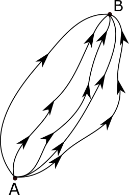
The path integral formulation is a description in quantum mechanics that generalizes the stationary action principle of classical mechanics. It replaces the classical notion of a single, unique classical trajectory for a system with a sum, or functional integral, over an infinity of quantum-mechanically possible trajectories to compute a quantum amplitude.
This formulation has proven crucial to the subsequent development of theoretical physics, because manifest Lorentz covariance (time and space components of quantities enter equations in the same way) is easier to achieve than in the operator formalism of canonical quantization. Unlike previous methods, the path integral allows one to easily change coordinates between very different canonical descriptions of the same quantum system. Another advantage is that it is in practice easier to guess the correct form of the Lagrangian of a theory, which naturally enters the path integrals (for interactions of a certain type, these are coordinate space or Feynman path integrals), than the Hamiltonian. Possible downsides of the approach include that unitarity (this is related to conservation of probability; the probabilities of all physically possible outcomes must add up to one) of the S-matrix is obscure in the formulation. The path-integral approach has proven to be equivalent to the other formalisms of quantum mechanics and quantum field theory. Thus, by deriving either approach from the other, problems associated with one or the other approach (as exemplified by Lorentz covariance or unitarity) go away.[1]
The path integral also relates quantum and stochastic processes, and this provided the basis for the grand synthesis of the 1970s, which unified quantum field theory with the statistical field theory of a fluctuating field near a second-order phase transition. The Schrödinger equation is a diffusion equation with an imaginary diffusion constant, and the path integral is an analytic continuation of a method for summing up all possible random walks.[2]
The path integral has impacted a wide array of sciences, including polymer physics, quantum field theory, string theory and cosmology. In physics, it is a foundation for lattice gauge theory and quantum chromodynamics.[3] It has been called the "most powerful formula in physics",[4] with Stephen Wolfram also declaring it to be the "fundamental mathematical construct of modern quantum mechanics and quantum field theory".[5]
The basic idea of the path integral formulation can be traced back to Norbert Wiener, who introduced the Wiener integral for solving problems in diffusion and Brownian motion.[6] This idea was extended to the use of the Lagrangian in quantum mechanics by Paul Dirac, whose 1933 paper gave birth to path integral formulation.[7][8][9][3] The complete method was developed in 1948 by Richard Feynman.[10] Some preliminaries were worked out earlier in his doctoral work under the supervision of John Archibald Wheeler. The original motivation stemmed from the desire to obtain a quantum-mechanical formulation for the Wheeler–Feynman absorber theory using a Lagrangian (rather than a Hamiltonian) as a starting point.

Quantum action principle
[edit]In quantum mechanics, as in classical mechanics, the Hamiltonian is the generator of time translations. This means that the state at a slightly later time differs from the state at the current time by the result of acting with the Hamiltonian operator (multiplied by the negative imaginary unit, −i). For states with a definite energy, this is a statement of the de Broglie relation between frequency and energy, and the general relation is consistent with that plus the superposition principle.
The Hamiltonian in classical mechanics is derived from a Lagrangian, which is a more fundamental quantity in the context of special relativity. The Hamiltonian indicates how to march forward in time, but the time is different in different reference frames. The Lagrangian is a Lorentz scalar, while the Hamiltonian is the time component of a four-vector. So the Hamiltonian is different in different frames, and this type of symmetry is not apparent in the original formulation of quantum mechanics.
The Hamiltonian is a function of the position and momentum at one time, and it determines the position and momentum a little later. The Lagrangian is a function of the position now and the position a little later (or, equivalently for infinitesimal time separations, it is a function of the position and velocity). The relation between the two is by a Legendre transformation, and the condition that determines the classical equations of motion (the Euler–Lagrange equations) is that the action has an extremum.
In quantum mechanics, the Legendre transform is hard to interpret, because the motion is not over a definite trajectory. In classical mechanics, with discretization in time, the Legendre transform becomes

and

where the partial derivative with respect to holds q(t + ε) fixed. The inverse Legendre transform is


where

and the partial derivative now is with respect to p at fixed q.
In quantum mechanics, the state is a superposition of different states with different values of q, or different values of p, and the quantities p and q can be interpreted as noncommuting operators. The operator p is only definite on states that are indefinite with respect to q. So consider two states separated in time and act with the operator corresponding to the Lagrangian:
![{\displaystyle e^{i{\big [}p{\big (}q(t+\varepsilon )-q(t){\big )}-\varepsilon H(p,q){\big ]}}.}](https://wikimedia.org/api/rest_v1/media/math/render/svg/612a1518d97cd3ba738de130868d805c22b46aff)
If the multiplications implicit in this formula are reinterpreted as matrix multiplications, the first factor is

and if this is also interpreted as a matrix multiplication, the sum over all states integrates over all q(t), and so it takes the Fourier transform in q(t) to change basis to p(t). That is the action on the Hilbert space – change basis to p at time t.
Next comes

or evolve an infinitesimal time into the future.
Finally, the last factor in this interpretation is

which means change basis back to q at a later time.
This is not very different from just ordinary time evolution: the H factor contains all the dynamical information – it pushes the state forward in time. The first part and the last part are just Fourier transforms to change to a pure q basis from an intermediate p basis.
Another way of saying this is that since the Hamiltonian is naturally a function of p and q, exponentiating this quantity and changing basis from p to q at each step allows the matrix element of H to be expressed as a simple function along each path. This function is the quantum analog of the classical action. This observation is due to Paul Dirac.[11]
Dirac further noted that one could square the time-evolution operator in the S representation:

and this gives the time-evolution operator between time t and time t + 2ε. While in the H representation the quantity that is being summed over the intermediate states is an obscure matrix element, in the S representation it is reinterpreted as a quantity associated to the path. In the limit that one takes a large power of this operator, one reconstructs the full quantum evolution between two states, the early one with a fixed value of q(0) and the later one with a fixed value of q(t). The result is a sum over paths with a phase, which is the quantum action.
Classical limit
[edit]Crucially, Dirac identified the effect of the classical limit on the quantum form of the action principle:
...we see that the integrand in (11) must be of the form eiF/h, where F is a function of qT, q1, q2, … qm, qt, which remains finite as h tends to zero. Let us now picture one of the intermediate qs, say qk, as varying continuously while the other ones are fixed. Owing to the smallness of h, we shall then in general have F/h varying extremely rapidly. This means that eiF/h will vary periodically with a very high frequency about the value zero, as a result of which its integral will be practically zero. The only important part in the domain of integration of qk is thus that for which a comparatively large variation in qk produces only a very small variation in F. This part is the neighbourhood of a point for which F is stationary with respect to small variations in qk. We can apply this argument to each of the variables of integration ... and obtain the result that the only important part in the domain of integration is that for which F is stationary for small variations in all intermediate qs. ... We see that F has for its classical analogue ∫t
T L dt, which is just the action function, which classical mechanics requires to be stationary for small variations in all the intermediate qs. This shows the way in which equation (11) goes over into classical results when h becomes extremely small.
— Dirac (1933), p. 69
That is, in the limit of action that is large compared to the Planck constant ħ – the classical limit – the path integral is dominated by solutions that are in the neighborhood of stationary points of the action. The classical path arises naturally in the classical limit.
Feynman's interpretation
[edit]Dirac's work did not provide a precise prescription to calculate the sum over paths, and he did not show that one could recover the Schrödinger equation or the canonical commutation relations from this rule. This was done by Feynman.
Feynman showed that Dirac's quantum action was, for most cases of interest, simply equal to the classical action, appropriately discretized. This means that the classical action is the phase acquired by quantum evolution between two fixed endpoints. He proposed to recover all of quantum mechanics from the following postulates:
- The probability for an event is given by the squared modulus of a complex number called the "probability amplitude".
- The probability amplitude is given by adding together the contributions of all paths in configuration space.
- The contribution of a path is proportional to eiS/ħ, where S is the action given by the time integral of the Lagrangian along the path.
In order to find the overall probability amplitude for a given process, then, one adds up, or integrates, the amplitude of the 3rd postulate over the space of all possible paths of the system in between the initial and final states, including those that are absurd by classical standards. In calculating the probability amplitude for a single particle to go from one space-time coordinate to another, it is correct to include paths in which the particle describes elaborate curlicues, curves in which the particle shoots off into outer space and flies back again, and so forth. The path integral assigns to all these amplitudes equal weight but varying phase, or argument of the complex number. Contributions from paths wildly different from the classical trajectory may be suppressed by interference (see below).
Feynman showed that this formulation of quantum mechanics is equivalent to the canonical approach to quantum mechanics when the Hamiltonian is at most quadratic in the momentum. An amplitude computed according to Feynman's principles will also obey the Schrödinger equation for the Hamiltonian corresponding to the given action.
The path integral formulation of quantum field theory represents the transition amplitude (corresponding to the classical correlation function) as a weighted sum of all possible histories of the system from the initial to the final state. A Feynman diagram is a graphical representation of a perturbative contribution to the transition amplitude.
Path integral in quantum mechanics
[edit]Time-slicing derivation
[edit]One common approach to deriving the path integral formula is to divide the time interval into small pieces. Once this is done, the Trotter product formula tells us that the noncommutativity of the kinetic and potential energy operators can be ignored.
For a particle in a smooth potential, the path integral is approximated by zigzag paths, which in one dimension is a product of ordinary integrals. For the motion of the particle from position xa at time ta to xb at time tb, the time sequence

can be divided up into n + 1 smaller segments tj − tj − 1, where j = 1, ..., n + 1, of fixed duration

This process is called time-slicing.[12]: 498
An approximation for the path integral can be computed as proportional to

where L(x, v) is the Lagrangian of the one-dimensional system with position variable x(t) and velocity v = ẋ(t) considered (see below), and dxj corresponds to the position at the jth time step, if the time integral is approximated by a sum of n terms.
In the limit n → ∞, this becomes a functional integral, which, apart from a nonessential factor, is directly the product of the probability amplitudes ⟨xb, tb|xa, ta⟩ (more precisely, since one must work with a continuous spectrum, the respective densities) to find the quantum mechanical particle at ta in the initial state xa and at tb in the final state xb.
Actually L is the classical Lagrangian of the one-dimensional system considered,

and the abovementioned "zigzagging" corresponds to the appearance of the terms

in the Riemann sum approximating the time integral, which are finally integrated over x1 to xn with the integration measure dx1...dxn, x̃j is an arbitrary value of the interval corresponding to j, e.g. its center, xj + xj−1/2.
Thus, in contrast to classical mechanics, not only does the stationary path contribute, but actually all virtual paths between the initial and the final point also contribute.
Path integral
[edit]In terms of the wave function in the position representation, the path integral formula reads as follows:
![{\displaystyle \psi (x,t)={\frac {1}{Z}}\int _{\mathbf {x} (0)=x}{\mathcal {D}}\mathbf {x} \,e^{iS[\mathbf {x} ,{\dot {\mathbf {x} }}]}\psi _{0}(\mathbf {x} (t))\,}](https://wikimedia.org/api/rest_v1/media/math/render/svg/63847726e284004a822be0b4d8210a8a713392c8)
where denotes integration over all paths with and where is a normalization factor. Here is the action, given by


![{\displaystyle S[\mathbf {x} ,{\dot {\mathbf {x} }}]=\int dt\,L(\mathbf {x} (t),{\dot {\mathbf {x} }}(t))}](https://wikimedia.org/api/rest_v1/media/math/render/svg/3b5011bdd160e07f4c3de4e918534275113f529f)
Free particle
[edit]The path integral representation gives the quantum amplitude to go from point x to point y as an integral over all paths. For a free-particle action (for simplicity let m = 1, ħ = 1)

the integral can be evaluated explicitly.
To do this, it is convenient to start without the factor i in the exponential, so that large deviations are suppressed by small numbers, not by cancelling oscillatory contributions. The amplitude (or Kernel) reads:

Splitting the integral into time slices:

where the D is interpreted as a finite collection of integrations at each integer multiple of ε. Each factor in the product is a Gaussian as a function of x(t + ε) centered at x(t) with variance ε. The multiple integrals are a repeated convolution of this Gaussian Gε with copies of itself at adjacent times:

where the number of convolutions is T/ε. The result is easy to evaluate by taking the Fourier transform of both sides, so that the convolutions become multiplications:

The Fourier transform of the Gaussian G is another Gaussian of reciprocal variance:

and the result is

The Fourier transform gives K, and it is a Gaussian again with reciprocal variance:

The proportionality constant is not really determined by the time-slicing approach, only the ratio of values for different endpoint choices is determined. The proportionality constant should be chosen to ensure that between each two time slices the time evolution is quantum-mechanically unitary, but a more illuminating way to fix the normalization is to consider the path integral as a description of a stochastic process.
The result has a probability interpretation. The sum over all paths of the exponential factor can be seen as the sum over each path of the probability of selecting that path. The probability is the product over each segment of the probability of selecting that segment, so that each segment is probabilistically independently chosen. The fact that the answer is a Gaussian spreading linearly in time is the central limit theorem, which can be interpreted as the first historical evaluation of a statistical path integral.
The probability interpretation gives a natural normalization choice. The path integral should be defined so that

This condition normalizes the Gaussian and produces a kernel that obeys the diffusion equation:

For oscillatory path integrals, ones with an i in the numerator, the time slicing produces convolved Gaussians, just as before. Now, however, the convolution product is marginally singular, since it requires careful limits to evaluate the oscillating integrals. To make the factors well defined, the easiest way is to add a small imaginary part to the time increment ε. This is closely related to Wick rotation. Then the same convolution argument as before gives the propagation kernel:

which, with the same normalization as before (not the sum-squares normalization – this function has a divergent norm), obeys a free Schrödinger equation:

This means that any superposition of Ks will also obey the same equation, by linearity. Defining

then ψt obeys the free Schrödinger equation just as K does:

Simple harmonic oscillator
[edit]The Lagrangian for the simple harmonic oscillator is[13]

Write its trajectory x(t) as the classical trajectory plus some perturbation, x(t) = xc(t) + δx(t) and the action as S = Sc + δS. The classical trajectory can be written as

This trajectory yields the classical action
![{\displaystyle {\begin{aligned}S_{\text{c}}&=\int _{t_{i}}^{t_{f}}{\mathcal {L}}\,dt=\int _{t_{i}}^{t_{f}}\left({\tfrac {1}{2}}m{\dot {x}}^{2}-{\tfrac {1}{2}}m\omega ^{2}x^{2}\right)\,dt\\[6pt]&={\frac {1}{2}}m\omega \left({\frac {(x_{i}^{2}+x_{f}^{2})\cos \omega (t_{f}-t_{i})-2x_{i}x_{f}}{\sin \omega (t_{f}-t_{i})}}\right)~.\end{aligned}}}](https://wikimedia.org/api/rest_v1/media/math/render/svg/045fbb738649f09823736e127c36f5082f118e84)
Next, expand the deviation from the classical path as a Fourier series, and calculate the contribution to the action δS, which gives

This means that the propagator is
![{\displaystyle {\begin{aligned}K(x_{f},t_{f};x_{i},t_{i})&=Qe^{\frac {iS_{\text{c}}}{\hbar }}\prod _{j=1}^{\infty }{\frac {j\pi }{\sqrt {2}}}\int da_{j}\exp {\left({\frac {i}{2\hbar }}a_{j}^{2}{\frac {m}{2}}\left({\frac {(j\pi )^{2}}{t_{f}-t_{i}}}-\omega ^{2}(t_{f}-t_{i})\right)\right)}\\[6pt]&=e^{\frac {iS_{\text{c}}}{\hbar }}Q\prod _{j=1}^{\infty }\left(1-\left({\frac {\omega (t_{f}-t_{i})}{j\pi }}\right)^{2}\right)^{-{\frac {1}{2}}}\end{aligned}}}](https://wikimedia.org/api/rest_v1/media/math/render/svg/4182856aaa82017672eff0d426a858a535e27d0b)
for some normalization

Using the infinite-product representation of the sinc function,

the propagator can be written as

Let T = tf − ti. One may write this propagator in terms of energy eigenstates as
![{\displaystyle {\begin{aligned}K(x_{f},t_{f};x_{i},t_{i})&=\left({\frac {m\omega }{2\pi i\hbar \sin \omega T}}\right)^{\frac {1}{2}}\exp {\left({\frac {i}{\hbar }}{\tfrac {1}{2}}m\omega {\frac {(x_{i}^{2}+x_{f}^{2})\cos \omega T-2x_{i}x_{f}}{\sin \omega T}}\right)}\\[6pt]&=\sum _{n=0}^{\infty }\exp {\left(-{\frac {iE_{n}T}{\hbar }}\right)}\psi _{n}(x_{f})\psi _{n}(x_{i})^{*}~.\end{aligned}}}](https://wikimedia.org/api/rest_v1/media/math/render/svg/f63c46394c38005de72cb1af4bec51b97aec548e)
Using the identities i sin ωT = 1/2eiωT (1 − e−2iωT) and cos ωT = 1/2eiωT (1 + e−2iωT), this amounts to

One may absorb all terms after the first e−iωT/2 into R(T), thereby obtaining

One may finally expand R(T) in powers of e−iωT: All terms in this expansion get multiplied by the e−iωT/2 factor in the front, yielding terms of the form

Comparison to the above eigenstate expansion yields the standard energy spectrum for the simple harmonic oscillator,

Coulomb potential
[edit]Feynman's time-sliced approximation does not, however, exist for the most important quantum-mechanical path integrals of atoms, due to the singularity of the Coulomb potential e2/r at the origin. Only after replacing the time t by another path-dependent pseudo-time parameter

the singularity is removed and a time-sliced approximation exists, which is exactly integrable, since it can be made harmonic by a simple coordinate transformation, as discovered in 1979 by İsmail Hakkı Duru and Hagen Kleinert.[14] The combination of a path-dependent time transformation and a coordinate transformation is an important tool to solve many path integrals and is called generically the Duru–Kleinert transformation.
The Schrödinger equation
[edit]The path integral reproduces the Schrödinger equation for the initial and final state even when a potential is present. This is easiest to see by taking a path-integral over infinitesimally separated times.

Since the time separation is infinitesimal and the cancelling oscillations become severe for large values of ẋ, the path integral has most weight for y close to x. In this case, to lowest order the potential energy is constant, and only the kinetic energy contribution is nontrivial. (This separation of the kinetic and potential energy terms in the exponent is essentially the Trotter product formula.) The exponential of the action is

The first term rotates the phase of ψ(x) locally by an amount proportional to the potential energy. The second term is the free particle propagator, corresponding to i times a diffusion process. To lowest order in ε they are additive; in any case one has with (1):

As mentioned, the spread in ψ is diffusive from the free particle propagation, with an extra infinitesimal rotation in phase that slowly varies from point to point from the potential:

and this is the Schrödinger equation. The normalization of the path integral needs to be fixed in exactly the same way as in the free particle case. An arbitrary continuous potential does not affect the normalization, although singular potentials require careful treatment.
Equations of motion
[edit]Since the states obey the Schrödinger equation, the path integral must reproduce the Heisenberg equations of motion for the averages of x and ẋ variables, but it is instructive to see this directly. The direct approach shows that the expectation values calculated from the path integral reproduce the usual ones of quantum mechanics.
Start by considering the path integral with some fixed initial state

Now x(t) at each separate time is a separate integration variable. So it is legitimate to change variables in the integral by shifting: x(t) = u(t) + ε(t) where ε(t) is a different shift at each time but ε(0) = ε(T) = 0, since the endpoints are not integrated:

The change in the integral from the shift is, to first infinitesimal order in ε:

which, integrating by parts in t, gives:

But this was just a shift of integration variables, which doesn't change the value of the integral for any choice of ε(t). The conclusion is that this first order variation is zero for an arbitrary initial state and at any arbitrary point in time:

this is the Heisenberg equation of motion.
If the action contains terms that multiply ẋ and x, at the same moment in time, the manipulations above are only heuristic, because the multiplication rules for these quantities is just as noncommuting in the path integral as it is in the operator formalism.
Stationary-phase approximation
[edit]If the variation in the action exceeds ħ by many orders of magnitude, we typically have destructive interference other than in the vicinity of those trajectories satisfying the Euler–Lagrange equation, which is now reinterpreted as the condition for constructive interference. This can be shown using the method of stationary phase applied to the propagator. As ħ decreases, the exponential in the integral oscillates rapidly in the complex domain for any change in the action. Thus, in the limit that ħ goes to zero, only points where the classical action does not vary contribute to the propagator.
Canonical commutation relations
[edit]The formulation of the path integral does not make it clear at first sight that the quantities x and p do not commute. In the path integral, these are just integration variables and they have no obvious ordering. Feynman discovered that the non-commutativity is still present.[15]
To see this, consider the simplest path integral, the brownian walk. This is not yet quantum mechanics, so in the path-integral the action is not multiplied by i:

The quantity x(t) is fluctuating, and the derivative is defined as the limit of a discrete difference.

The distance that a random walk moves is proportional to √t, so that:

This shows that the random walk is not differentiable, since the ratio that defines the derivative diverges with probability one.
The quantity xẋ is ambiguous, with two possible meanings:
![{\displaystyle [1]=x{\frac {dx}{dt}}=x(t){\frac {x(t+\varepsilon )-x(t)}{\varepsilon }}}](https://wikimedia.org/api/rest_v1/media/math/render/svg/ec8f251860d68e9e7f988d44fd900c0a91e48e8b)
![{\displaystyle [2]=x{\frac {dx}{dt}}=x(t+\varepsilon ){\frac {x(t+\varepsilon )-x(t)}{\varepsilon }}}](https://wikimedia.org/api/rest_v1/media/math/render/svg/299c595d865a660a326c75e3c627e2077126c765)
In elementary calculus, the two are only different by an amount that goes to 0 as ε goes to 0. But in this case, the difference between the two is not 0:
![{\displaystyle [2]-[1]={\frac {{\big (}x(t+\varepsilon )-x(t){\big )}^{2}}{\varepsilon }}\approx {\frac {\varepsilon }{\varepsilon }}}](https://wikimedia.org/api/rest_v1/media/math/render/svg/c987304e52bfa1dadac2aab1c402035017a524c8)
Let

Then f(t) is a rapidly fluctuating statistical quantity, whose average value is 1, i.e. a normalized "Gaussian process". The fluctuations of such a quantity can be described by a statistical Lagrangian

and the equations of motion for f derived from extremizing the action S corresponding to L just set it equal to 1. In physics, such a quantity is "equal to 1 as an operator identity". In mathematics, it "weakly converges to 1". In either case, it is 1 in any expectation value, or when averaged over any interval, or for all practical purpose.
Defining the time order to be the operator order:
![{\displaystyle [x,{\dot {x}}]=x{\frac {dx}{dt}}-{\frac {dx}{dt}}x=1}](https://wikimedia.org/api/rest_v1/media/math/render/svg/d3a27062611afdbf93bdf30d31f8a003633c25c1)
This is called the Itō lemma in stochastic calculus, and the (euclideanized) canonical commutation relations in physics.
For a general statistical action, a similar argument shows that
![{\displaystyle \left[x,{\frac {\partial S}{\partial {\dot {x}}}}\right]=1}](https://wikimedia.org/api/rest_v1/media/math/render/svg/c068c9f75efe46dc8da5b8154c2c6b524f81baff)
and in quantum mechanics, the extra imaginary unit in the action converts this to the canonical commutation relation,
![{\displaystyle [x,p]=i}](https://wikimedia.org/api/rest_v1/media/math/render/svg/68322d6a3131d29b89c3b525d5380b219a220821)
Particle in curved space
[edit]For a particle in curved space the kinetic term depends on the position, and the above time slicing cannot be applied, this being a manifestation of the notorious operator ordering problem in Schrödinger quantum mechanics. One may, however, solve this problem by transforming the time-sliced flat-space path integral to curved space using a multivalued coordinate transformation (nonholonomic mapping explained here).
Measure-theoretic factors
[edit]Sometimes (e.g. a particle moving in curved space) we also have measure-theoretic factors in the functional integral:
![{\displaystyle \int \mu [x]e^{iS[x]}\,{\mathcal {D}}x.}](https://wikimedia.org/api/rest_v1/media/math/render/svg/751ff6cb46202a7a93d1d0735da68ec9883b1f94)
This factor is needed to restore unitarity.
For instance, if

then it means that each spatial slice is multiplied by the measure √g. This measure cannot be expressed as a functional multiplying the Dx measure because they belong to entirely different classes.
Expectation values and matrix elements
[edit]Matrix elements of the kind take the form

- .
![{\displaystyle \int _{x(0)=x_{i}}^{x(t)=x_{f}}{\mathcal {D}}[x]F(x(t'))e^{{\frac {i}{\hbar }}\int dtL(x(t),{\dot {x}}(t))}}](https://wikimedia.org/api/rest_v1/media/math/render/svg/67d451d6c7235252420f0e3fa8adb5960e61ec43)
This generalizes to multiple operators, for example
- ,
![{\displaystyle \langle x_{f}|e^{-{\frac {i}{\hbar }}{\hat {H}}(t-t_{1})}F_{1}({\hat {x}})e^{-{\frac {i}{\hbar }}{\hat {H}}(t_{1}-t_{2})}F_{2}({\hat {x}})e^{-{\frac {i}{\hbar }}{\hat {H}}(t_{2})}|x_{i}\rangle =\int _{x(0)=x_{i}}^{x(t)=x_{f}}{\mathcal {D}}[x]F_{1}(x(t_{1}))F_{2}(x(t_{2}))e^{{\frac {i}{\hbar }}\int dtL(x(t),{\dot {x}}(t))}}](https://wikimedia.org/api/rest_v1/media/math/render/svg/55b8e00db6a2ef338d85b7542a7e8abe3ac8cf16)
and to the general vacuum expectation value (in the large time limit)
- .
![{\displaystyle \langle F\rangle ={\frac {\int {\mathcal {D}}[\phi ]F(\phi )e^{{\frac {i}{\hbar }}S[\phi ]}}{\int {\mathcal {D}}[\phi ]e^{{\frac {i}{\hbar }}S[\phi ]}}}}](https://wikimedia.org/api/rest_v1/media/math/render/svg/e5cde79b9d454bfe5f02829e19906c80cdcaa392)
Euclidean path integrals
[edit]It is very common in path integrals to perform a Wick rotation from real to imaginary times. In the setting of quantum field theory, the Wick rotation changes the geometry of space-time from Lorentzian to Euclidean; as a result, Wick-rotated path integrals are often called Euclidean path integrals.
Wick rotation and the Feynman–Kac formula
[edit]If we replace by , the time-evolution operator is replaced by . (This change is known as a Wick rotation.) If we repeat the derivation of the path-integral formula in this setting, we obtain[16]


- ,

where is the Euclidean action, given by

- .
![{\displaystyle S_{\mathrm {Euclidean} }(\mathbf {x} ,{\dot {\mathbf {x} }})=\int \left[{\frac {m}{2}}|{\dot {\mathbf {x} }}(t)|^{2}+V(\mathbf {x} (t))\right]\,dt}](https://wikimedia.org/api/rest_v1/media/math/render/svg/9aa1dbe41729019d2dd493ceaec5fa7c73a2553c)
Note the sign change between this and the normal action, where the potential energy term is negative. (The term Euclidean is from the context of quantum field theory, where the change from real to imaginary time changes the space-time geometry from Lorentzian to Euclidean.)
Now, the contribution of the kinetic energy to the path integral is as follows:

where includes all the remaining dependence of the integrand on the path. This integral has a rigorous mathematical interpretation as integration against the Wiener measure, denoted . The Wiener measure, constructed by Norbert Wiener gives a rigorous foundation to Einstein's mathematical model of Brownian motion. The subscript indicates that the measure is supported on paths with .


We then have a rigorous version of the Feynman path integral, known as the Feynman–Kac formula:[17]
- ,

where now satisfies the Wick-rotated version of the Schrödinger equation,

- .

Although the Wick-rotated Schrödinger equation does not have a direct physical meaning, interesting properties of the Schrödinger operator can be extracted by studying it.[18]

Much of the study of quantum field theories from the path-integral perspective, in both the mathematics and physics literatures, is done in the Euclidean setting, that is, after a Wick rotation. In particular, there are various results showing that if a Euclidean field theory with suitable properties can be constructed, one can then undo the Wick rotation to recover the physical, Lorentzian theory.[19] On the other hand, it is much more difficult to give a meaning to path integrals (even Euclidean path integrals) in quantum field theory than in quantum mechanics.[20]
Path integral and the partition function
[edit]The path integral is just the generalization of the integral above to all quantum mechanical problems—
![{\displaystyle Z=\int e^{\frac {i{\mathcal {S}}[\mathbf {x} ]}{\hbar }}\,{\mathcal {D}}\mathbf {x} \quad {\text{where }}{\mathcal {S}}[\mathbf {x} ]=\int _{0}^{t_{f}}L[\mathbf {x} (t),{\dot {\mathbf {x} }}(t)]\,dt}](https://wikimedia.org/api/rest_v1/media/math/render/svg/4081ea7aee92bd8923f1300d76a3ab2e2f0dfd72)
is the action of the classical problem in which one investigates the path starting at time t = 0 and ending at time t = tf, and denotes the integration measure over all paths. In the classical limit, , the path of minimum action dominates the integral, because the phase of any path away from this fluctuates rapidly and different contributions cancel.[21]
![{\displaystyle {\mathcal {S}}[\mathbf {x} ]\gg \hbar }](https://wikimedia.org/api/rest_v1/media/math/render/svg/63becd74c8345f71aa038ebbe0c1dd5a173d8c37)
The connection with statistical mechanics follows. Considering only paths that begin and end in the same configuration, perform the Wick rotation it = ħβ, i.e., make time imaginary, and integrate over all possible beginning-ending configurations. The Wick-rotated path integral—described in the previous subsection, with the ordinary action replaced by its "Euclidean" counterpart—now resembles the partition function of statistical mechanics defined in a canonical ensemble with inverse temperature proportional to imaginary time, 1/T = ikBt/ħ. Strictly speaking, though, this is the partition function for a statistical field theory.
Clearly, such a deep analogy between quantum mechanics and statistical mechanics cannot be dependent on the formulation. In the canonical formulation, one sees that the unitary evolution operator of a state is given by

where the state α is evolved from time t = 0. If one makes a Wick rotation here, and finds the amplitude to go from any state, back to the same state in (imaginary) time iβ is given by
![{\displaystyle Z=\operatorname {Tr} \left[e^{-H\beta }\right]}](https://wikimedia.org/api/rest_v1/media/math/render/svg/c392558011f101562fa6ffd0c6d9c53a22f830ee)
which is precisely the partition function of statistical mechanics for the same system at the temperature quoted earlier. One aspect of this equivalence was also known to Erwin Schrödinger who remarked that the equation named after him looked like the diffusion equation after Wick rotation. Note, however, that the Euclidean path integral is actually in the form of a classical statistical mechanics model.
Quantum field theory
[edit]| Quantum field theory |
|---|
 |
| History |
Both the Schrödinger and Heisenberg approaches to quantum mechanics single out time and are not in the spirit of relativity. For example, the Heisenberg approach requires that scalar field operators obey the commutation relation
![{\displaystyle [\varphi (x),\partial _{t}\varphi (y)]=i\delta ^{3}(x-y)}](https://wikimedia.org/api/rest_v1/media/math/render/svg/e0dd61e9a1a73f935161139e2d89278803d7d99f)
for two simultaneous spatial positions x and y, and this is not a relativistically invariant concept. The results of a calculation are covariant, but the symmetry is not apparent in intermediate stages. If naive field-theory calculations did not produce infinite answers in the continuum limit, this would not have been such a big problem – it would just have been a bad choice of coordinates. But the lack of symmetry means that the infinite quantities must be cut off, and the bad coordinates make it nearly impossible to cut off the theory without spoiling the symmetry. This makes it difficult to extract the physical predictions, which require a careful limiting procedure.
The problem of lost symmetry also appears in classical mechanics, where the Hamiltonian formulation also superficially singles out time. The Lagrangian formulation makes the relativistic invariance apparent. In the same way, the path integral is manifestly relativistic. It reproduces the Schrödinger equation, the Heisenberg equations of motion, and the canonical commutation relations and shows that they are compatible with relativity. It extends the Heisenberg-type operator algebra to operator product rules, which are new relations difficult to see in the old formalism.
Further, different choices of canonical variables lead to very different-seeming formulations of the same theory. The transformations between the variables can be very complicated, but the path integral makes them into reasonably straightforward changes of integration variables. For these reasons, the Feynman path integral has made earlier formalisms largely obsolete.
The price of a path integral representation is that the unitarity of a theory is no longer self-evident, but it can be proven by changing variables to some canonical representation. The path integral itself also deals with larger mathematical spaces than is usual, which requires more careful mathematics, not all of which has been fully worked out. The path integral historically was not immediately accepted, partly because it took many years to incorporate fermions properly. This required physicists to invent an entirely new mathematical object – the Grassmann variable – which also allowed changes of variables to be done naturally, as well as allowing constrained quantization.
The integration variables in the path integral are subtly non-commuting. The value of the product of two field operators at what looks like the same point depends on how the two points are ordered in space and time. This makes some naive identities fail.
Propagator
[edit]In relativistic theories, there is both a particle and field representation for every theory. The field representation is a sum over all field configurations, and the particle representation is a sum over different particle paths.
The nonrelativistic formulation is traditionally given in terms of particle paths, not fields. There, the path integral in the usual variables, with fixed boundary conditions, gives the probability amplitude for a particle to go from point x to point y in time T:
![{\displaystyle K(x,y;T)=\langle y;T\mid x;0\rangle =\int _{x(0)=x}^{x(T)=y}e^{iS[x]}\,Dx.}](https://wikimedia.org/api/rest_v1/media/math/render/svg/13a2490ba92f4528eac85157f3af098d2b480c11)
This is called the propagator. To obtain the final state at y we simply apply K(x,y; T) to the initial state and integrate over x resulting in:
![{\displaystyle \psi _{T}(y)=\int _{x}\psi _{0}(x)K(x,y;T)\,dx=\int ^{x(T)=y}\psi _{0}(x(0))e^{iS[x]}\,Dx.}](https://wikimedia.org/api/rest_v1/media/math/render/svg/d99e0c051b9f404b3a46ec79d4913270c62448ab)
For a spatially homogeneous system, where K(x, y) is only a function of (x − y), the integral is a convolution, the final state is the initial state convolved with the propagator:

For a free particle of mass m, the propagator can be evaluated either explicitly from the path integral or by noting that the Schrödinger equation is a diffusion equation in imaginary time, and the solution must be a normalized Gaussian:

Taking the Fourier transform in (x − y) produces another Gaussian:

and in p-space the proportionality factor here is constant in time, as will be verified in a moment. The Fourier transform in time, extending K(p; T) to be zero for negative times, gives Green's function, or the frequency-space propagator:

which is the reciprocal of the operator that annihilates the wavefunction in the Schrödinger equation, which wouldn't have come out right if the proportionality factor weren't constant in the p-space representation.
The infinitesimal term in the denominator is a small positive number, which guarantees that the inverse Fourier transform in E will be nonzero only for future times. For past times, the inverse Fourier transform contour closes toward values of E where there is no singularity. This guarantees that K propagates the particle into the future and is the reason for the subscript "F" on G. The infinitesimal term can be interpreted as an infinitesimal rotation toward imaginary time.
It is also possible to reexpress the nonrelativistic time evolution in terms of propagators going toward the past, since the Schrödinger equation is time-reversible. The past propagator is the same as the future propagator except for the obvious difference that it vanishes in the future, and in the Gaussian t is replaced by −t. In this case, the interpretation is that these are the quantities to convolve the final wavefunction so as to get the initial wavefunction:

Given the nearly identical only change is the sign of E and ε, the parameter E in Green's function can either be the energy if the paths are going toward the future, or the negative of the energy if the paths are going toward the past.
For a nonrelativistic theory, the time as measured along the path of a moving particle and the time as measured by an outside observer are the same. In relativity, this is no longer true. For a relativistic theory the propagator should be defined as the sum over all paths that travel between two points in a fixed proper time, as measured along the path (these paths describe the trajectory of a particle in space and in time):

The integral above is not trivial to interpret because of the square root. Fortunately, there is a heuristic trick. The sum is over the relativistic arc length of the path of an oscillating quantity, and like the nonrelativistic path integral should be interpreted as slightly rotated into imaginary time. The function K(x − y, τ) can be evaluated when the sum is over paths in Euclidean space:

This describes a sum over all paths of length Τ of the exponential of minus the length. This can be given a probability interpretation. The sum over all paths is a probability average over a path constructed step by step. The total number of steps is proportional to Τ, and each step is less likely the longer it is. By the central limit theorem, the result of many independent steps is a Gaussian of variance proportional to Τ:

The usual definition of the relativistic propagator only asks for the amplitude to travel from x to y, after summing over all the possible proper times it could take:

where W(Τ) is a weight factor, the relative importance of paths of different proper time. By the translation symmetry in proper time, this weight can only be an exponential factor and can be absorbed into the constant α:

This is the Schwinger representation. Taking a Fourier transform over the variable (x − y) can be done for each value of Τ separately, and because each separate Τ contribution is a Gaussian, gives whose Fourier transform is another Gaussian with reciprocal width. So in p-space, the propagator can be reexpressed simply:

which is the Euclidean propagator for a scalar particle. Rotating p0 to be imaginary gives the usual relativistic propagator, up to a factor of −i and an ambiguity, which will be clarified below:

This expression can be interpreted in the nonrelativistic limit, where it is convenient to split it by partial fractions:

For states where one nonrelativistic particle is present, the initial wavefunction has a frequency distribution concentrated near p0 = m. When convolving with the propagator, which in p space just means multiplying by the propagator, the second term is suppressed and the first term is enhanced. For frequencies near p0 = m, the dominant first term has the form

This is the expression for the nonrelativistic Green's function of a free Schrödinger particle.
The second term has a nonrelativistic limit also, but this limit is concentrated on frequencies that are negative. The second pole is dominated by contributions from paths where the proper time and the coordinate time are ticking in an opposite sense, which means that the second term is to be interpreted as the antiparticle. The nonrelativistic analysis shows that with this form the antiparticle still has positive energy.
The proper way to express this mathematically is that, adding a small suppression factor in proper time, the limit where t → −∞ of the first term must vanish, while the t → +∞ limit of the second term must vanish. In the Fourier transform, this means shifting the pole in p0 slightly, so that the inverse Fourier transform will pick up a small decay factor in one of the time directions:

Without these terms, the pole contribution could not be unambiguously evaluated when taking the inverse Fourier transform of p0. The terms can be recombined:

which when factored, produces opposite-sign infinitesimal terms in each factor. This is the mathematically precise form of the relativistic particle propagator, free of any ambiguities. The ε term introduces a small imaginary part to the α = m2, which in the Minkowski version is a small exponential suppression of long paths.
So in the relativistic case, the Feynman path-integral representation of the propagator includes paths going backwards in time, which describe antiparticles. The paths that contribute to the relativistic propagator go forward and backwards in time, and the interpretation of this is that the amplitude for a free particle to travel between two points includes amplitudes for the particle to fluctuate into an antiparticle, travel back in time, then forward again.
Unlike the nonrelativistic case, it is impossible to produce a relativistic theory of local particle propagation without including antiparticles. All local differential operators have inverses that are nonzero outside the light cone, meaning that it is impossible to keep a particle from travelling faster than light. Such a particle cannot have a Green's function that is only nonzero in the future in a relativistically invariant theory.
Functionals of fields
[edit]However, the path integral formulation is also extremely important in direct application to quantum field theory, in which the "paths" or histories being considered are not the motions of a single particle, but the possible time evolutions of a field over all space. The action is referred to technically as a functional of the field: S[ϕ], where the field ϕ(xμ) is itself a function of space and time, and the square brackets are a reminder that the action depends on all the field's values everywhere, not just some particular value. One such given function ϕ(xμ) of spacetime is called a field configuration. In principle, one integrates Feynman's amplitude over the class of all possible field configurations.
Much of the formal study of QFT is devoted to the properties of the resulting functional integral, and much effort (not yet entirely successful) has been made toward making these functional integrals mathematically precise.
Such a functional integral is extremely similar to the partition function in statistical mechanics. Indeed, it is sometimes called a partition function, and the two are essentially mathematically identical except for the factor of i in the exponent in Feynman's postulate 3. Analytically continuing the integral to an imaginary time variable (called a Wick rotation) makes the functional integral even more like a statistical partition function and also tames some of the mathematical difficulties of working with these integrals.
Expectation values
[edit]In quantum field theory, if the action is given by the functional S of field configurations (which only depends locally on the fields), then the time-ordered vacuum expectation value of polynomially bounded functional F, ⟨F⟩, is given by
![{\displaystyle \langle F\rangle ={\frac {\int {\mathcal {D}}\varphi F[\varphi ]e^{i{\mathcal {S}}[\varphi ]}}{\int {\mathcal {D}}\varphi e^{i{\mathcal {S}}[\varphi ]}}}.}](https://wikimedia.org/api/rest_v1/media/math/render/svg/c8dd3d8f7f56934dd5dc162ad33111913bac8a96)
The symbol ∫Dϕ here is a concise way to represent the infinite-dimensional integral over all possible field configurations on all of space-time. As stated above, the unadorned path integral in the denominator ensures proper normalization.
As a probability
[edit]Strictly speaking, the only question that can be asked in physics is: What fraction of states satisfying condition A also satisfy condition B? The answer to this is a number between 0 and 1, which can be interpreted as a conditional probability, written as P(B|A). In terms of path integration, since P(B|A) = P(A∩B) / P(A), this means
![{\displaystyle \operatorname {P} (B\mid A)={\frac {\sum _{F\subset A\cap B}\left|\int {\mathcal {D}}\varphi O_{\text{in}}[\varphi ]e^{i{\mathcal {S}}[\varphi ]}F[\varphi ]\right|^{2}}{\sum _{F\subset A}\left|\int {\mathcal {D}}\varphi O_{\text{in}}[\varphi ]e^{i{\mathcal {S}}[\varphi ]}F[\varphi ]\right|^{2}}},}](https://wikimedia.org/api/rest_v1/media/math/render/svg/ae50ce50d99fed4b30b60f1abd8bd23bfc21227a)
where the functional Oin[ϕ] is the superposition of all incoming states that could lead to the states we are interested in. In particular, this could be a state corresponding to the state of the Universe just after the Big Bang, although for actual calculation this can be simplified using heuristic methods. Since this expression is a quotient of path integrals, it is naturally normalised.
Schwinger–Dyson equations
[edit]Since this formulation of quantum mechanics is analogous to classical action principle, one might expect that identities concerning the action in classical mechanics would have quantum counterparts derivable from a functional integral. This is often the case.
In the language of functional analysis, we can write the Euler–Lagrange equations as
![{\displaystyle {\frac {\delta {\mathcal {S}}[\varphi ]}{\delta \varphi }}=0}](https://wikimedia.org/api/rest_v1/media/math/render/svg/bfb4de731adf904b88deade6b70258828ed4f09b)
(the left-hand side is a functional derivative; the equation means that the action is stationary under small changes in the field configuration). The quantum analogues of these equations are called the Schwinger–Dyson equations.
If the functional measure Dϕ turns out to be translationally invariant (we'll assume this for the rest of this article, although this does not hold for, let's say nonlinear sigma models), and if we assume that after a Wick rotation
![{\displaystyle e^{i{\mathcal {S}}[\varphi ]},}](https://wikimedia.org/api/rest_v1/media/math/render/svg/72853bae20ab0e1b75f33011ada66f826ecab088)
which now becomes
![{\displaystyle e^{-H[\varphi ]}}](https://wikimedia.org/api/rest_v1/media/math/render/svg/569838b0b4ff05dc6e23bc07778f9f962fcfd243)
for some H, it goes to zero faster than a reciprocal of any polynomial for large values of φ, then we can integrate by parts (after a Wick rotation, followed by a Wick rotation back) to get the following Schwinger–Dyson equations for the expectation:
![{\displaystyle \left\langle {\frac {\delta F[\varphi ]}{\delta \varphi }}\right\rangle =-i\left\langle F[\varphi ]{\frac {\delta {\mathcal {S}}[\varphi ]}{\delta \varphi }}\right\rangle }](https://wikimedia.org/api/rest_v1/media/math/render/svg/0ab0605db250f78b7a72d8c9a8be5ea981e98938)
for any polynomially-bounded functional F. In the deWitt notation this looks like[22]

These equations are the analog of the on-shell EL equations. The time ordering is taken before the time derivatives inside the S,i.
If J (called the source field) is an element of the dual space of the field configurations (which has at least an affine structure because of the assumption of the translational invariance for the functional measure), then the generating functional Z of the source fields is defined to be
![{\displaystyle Z[J]=\int {\mathcal {D}}\varphi e^{i\left({\mathcal {S}}[\varphi ]+\langle J,\varphi \rangle \right)}.}](https://wikimedia.org/api/rest_v1/media/math/render/svg/5c0bb94dfefb303272fe0566a3d021312ac35966)
Note that
![{\displaystyle {\frac {\delta ^{n}Z}{\delta J(x_{1})\cdots \delta J(x_{n})}}[J]=i^{n}\,Z[J]\,\left\langle \varphi (x_{1})\cdots \varphi (x_{n})\right\rangle _{J},}](https://wikimedia.org/api/rest_v1/media/math/render/svg/51ad1e13e298e27ca37cea282dfb558ada113de9)
or
![{\displaystyle Z^{,i_{1}\cdots i_{n}}[J]=i^{n}Z[J]\left\langle \varphi ^{i_{1}}\cdots \varphi ^{i_{n}}\right\rangle _{J},}](https://wikimedia.org/api/rest_v1/media/math/render/svg/d1b4fbd7299210e2c476c87216723801b4cdefbb)
where
![{\displaystyle \langle F\rangle _{J}={\frac {\int {\mathcal {D}}\varphi F[\varphi ]e^{i\left({\mathcal {S}}[\varphi ]+\langle J,\varphi \rangle \right)}}{\int {\mathcal {D}}\varphi e^{i\left({\mathcal {S}}[\varphi ]+\langle J,\varphi \rangle \right)}}}.}](https://wikimedia.org/api/rest_v1/media/math/render/svg/ee5557cbd2cdb86590e7c666b51770fcc80d6ecb)
Basically, if Dφ eiS[φ] is viewed as a functional distribution (this shouldn't be taken too literally as an interpretation of QFT, unlike its Wick-rotated statistical mechanics analogue, because we have time ordering complications here!), then ⟨φ(x1) ... φ(xn)⟩ are its moments, and Z is its Fourier transform.
If F is a functional of φ, then for an operator K, F[K] is defined to be the operator that substitutes K for φ. For example, if
![{\displaystyle F[\varphi ]={\frac {\partial ^{k_{1}}}{\partial x_{1}^{k_{1}}}}\varphi (x_{1})\cdots {\frac {\partial ^{k_{n}}}{\partial x_{n}^{k_{n}}}}\varphi (x_{n}),}](https://wikimedia.org/api/rest_v1/media/math/render/svg/4cfaa9b6dbc2a4f700fedbf508daffb46857b8c7)
and G is a functional of J, then
![{\displaystyle F\left[-i{\frac {\delta }{\delta J}}\right]G[J]=(-i)^{n}{\frac {\partial ^{k_{1}}}{\partial x_{1}^{k_{1}}}}{\frac {\delta }{\delta J(x_{1})}}\cdots {\frac {\partial ^{k_{n}}}{\partial x_{n}^{k_{n}}}}{\frac {\delta }{\delta J(x_{n})}}G[J].}](https://wikimedia.org/api/rest_v1/media/math/render/svg/4b809c494c78617b22f3a7eb51229916366f3bee)
Then, from the properties of the functional integrals
![{\displaystyle \left\langle {\frac {\delta {\mathcal {S}}}{\delta \varphi (x)}}[\varphi ]+J(x)\right\rangle _{J}=0}](https://wikimedia.org/api/rest_v1/media/math/render/svg/eacbb7505e8ede2b17344cd5da8021c52f05e1d3)
we get the "master" Schwinger–Dyson equation:
![{\displaystyle {\frac {\delta {\mathcal {S}}}{\delta \varphi (x)}}\left[-i{\frac {\delta }{\delta J}}\right]Z[J]+J(x)Z[J]=0,}](https://wikimedia.org/api/rest_v1/media/math/render/svg/c943233dae4175a4d8c19052414ab8cc7a58bd31)
or
![{\displaystyle {\mathcal {S}}_{,i}[-i\partial ]Z+J_{i}Z=0.}](https://wikimedia.org/api/rest_v1/media/math/render/svg/4f80fc729f6339c28c610ea01f6ebbc39c954e43)
If the functional measure is not translationally invariant, it might be possible to express it as the product M[φ] Dφ, where M is a functional and Dφ is a translationally invariant measure. This is true, for example, for nonlinear sigma models where the target space is diffeomorphic to Rn. However, if the target manifold is some topologically nontrivial space, the concept of a translation does not even make any sense.
In that case, we would have to replace the S in this equation by another functional

If we expand this equation as a Taylor series about J = 0, we get the entire set of Schwinger–Dyson equations.
Localization
[edit]The path integrals are usually thought of as being the sum of all paths through an infinite space–time. However, in local quantum field theory we would restrict everything to lie within a finite causally complete region, for example inside a double light-cone. This gives a more mathematically precise and physically rigorous definition of quantum field theory.
Ward–Takahashi identities
[edit]Now how about the on shell Noether's theorem for the classical case? Does it have a quantum analog as well? Yes, but with a caveat. The functional measure would have to be invariant under the one parameter group of symmetry transformation as well.
Let's just assume for simplicity here that the symmetry in question is local (not local in the sense of a gauge symmetry, but in the sense that the transformed value of the field at any given point under an infinitesimal transformation would only depend on the field configuration over an arbitrarily small neighborhood of the point in question). Let's also assume that the action is local in the sense that it is the integral over spacetime of a Lagrangian, and that
![{\displaystyle Q[{\mathcal {L}}(x)]=\partial _{\mu }f^{\mu }(x)}](https://wikimedia.org/api/rest_v1/media/math/render/svg/783dfeb077d75c74001b16901af455cdcee9739a)
for some function f where f only depends locally on φ (and possibly the spacetime position).
If we don't assume any special boundary conditions, this would not be a "true" symmetry in the true sense of the term in general unless f = 0 or something. Here, Q is a derivation that generates the one parameter group in question. We could have antiderivations as well, such as BRST and supersymmetry.
Let's also assume
![{\displaystyle \int {\mathcal {D}}\varphi \,Q[F][\varphi ]=0}](https://wikimedia.org/api/rest_v1/media/math/render/svg/a938d847265651ecf1e7da4508e8bae8bdac5961)
for any polynomially-bounded functional F. This property is called the invariance of the measure, and this does not hold in general. (See anomaly (physics) for more details.)
Then,
![{\displaystyle \int {\mathcal {D}}\varphi \,Q\left[Fe^{iS}\right][\varphi ]=0,}](https://wikimedia.org/api/rest_v1/media/math/render/svg/1dfd63c0fd16df415605732e39e93ac92b70969c)
which implies
![{\displaystyle \langle Q[F]\rangle +i\left\langle F\int _{\partial V}f^{\mu }\,ds_{\mu }\right\rangle =0}](https://wikimedia.org/api/rest_v1/media/math/render/svg/cc0bdaaad1763e314c753caf7a59ec37fb6dba32)
where the integral is over the boundary. This is the quantum analog of Noether's theorem.
Now, let's assume even further that Q is a local integral

where
![{\displaystyle q(x)[\varphi (y)]=\delta ^{(d)}(X-y)Q[\varphi (y)]\,}](https://wikimedia.org/api/rest_v1/media/math/render/svg/025974d6d70aca94e21a0324d78ff850a5d7741a)
so that\
![{\displaystyle q(x)[S]=\partial _{\mu }j^{\mu }(x)\,}](https://wikimedia.org/api/rest_v1/media/math/render/svg/5e24e0482aaf028b21c9706779595151eba65129)
where
![{\displaystyle j^{\mu }(x)=f^{\mu }(x)-{\frac {\partial }{\partial (\partial _{\mu }\varphi )}}{\mathcal {L}}(x)Q[\varphi ]\,}](https://wikimedia.org/api/rest_v1/media/math/render/svg/0b0d2f4b2a1a3bf0c05e419d2faf62fb3b6d2301)
(this is assuming the Lagrangian only depends on φ and its first partial derivatives! More general Lagrangians would require a modification to this definition!). We're not insisting that q(x) is the generator of a symmetry (i.e. we are not insisting upon the gauge principle), but just that Q is. And we also assume the even stronger assumption that the functional measure is locally invariant:
![{\displaystyle \int {\mathcal {D}}\varphi \,q(x)[F][\varphi ]=0.}](https://wikimedia.org/api/rest_v1/media/math/render/svg/ab340dbb8a6c70857e63053f5126bfcb8e5efd23)
Then, we would have
![{\displaystyle \langle q(x)[F]\rangle +i\langle Fq(x)[S]\rangle =\langle q(x)[F]\rangle +i\left\langle F\partial _{\mu }j^{\mu }(x)\right\rangle =0.}](https://wikimedia.org/api/rest_v1/media/math/render/svg/cd258e91dd9d104cbda7c100b7a3051c3a182699)
Alternatively,
![{\displaystyle q(x)[S]\left[-i{\frac {\delta }{\delta J}}\right]Z[J]+J(x)Q[\varphi (x)]\left[-i{\frac {\delta }{\delta J}}\right]Z[J]=\partial _{\mu }j^{\mu }(x)\left[-i{\frac {\delta }{\delta J}}\right]Z[J]+J(x)Q[\varphi (x)]\left[-i{\frac {\delta }{\delta J}}\right]Z[J]=0.}](https://wikimedia.org/api/rest_v1/media/math/render/svg/7a5d0cb54c839fe82d7a5030dfb1455dc0b610bd)
The above two equations are the Ward–Takahashi identities.
Now for the case where f = 0, we can forget about all the boundary conditions and locality assumptions. We'd simply have
![{\displaystyle \left\langle Q[F]\right\rangle =0.}](https://wikimedia.org/api/rest_v1/media/math/render/svg/afdc3e73929181acdd9426370f11dc3d12db08cc)
Alternatively,
![{\displaystyle \int d^{d}x\,J(x)Q[\varphi (x)]\left[-i{\frac {\delta }{\delta J}}\right]Z[J]=0.}](https://wikimedia.org/api/rest_v1/media/math/render/svg/cda2802a1efe3f726404ca358543487fb48fd119)
Caveats
[edit]Need for regulators and renormalization
[edit]Path integrals as they are defined here require the introduction of regulators. Changing the scale of the regulator leads to the renormalization group. In fact, renormalization is the major obstruction to making path integrals well-defined.
Ordering prescription
[edit]Regardless of whether one works in configuration space or phase space, when equating the operator formalism and the path integral formulation, an ordering prescription is required to resolve the ambiguity in the correspondence between non-commutative operators and the commutative functions that appear in path integrands. For example, the operator can be translated back as either , , or depending on whether one chooses the , , or Weyl ordering prescription; conversely, can be translated to either , , or for the same respective choice of ordering prescription.


Path integral in quantum-mechanical interpretation
[edit]In one interpretation of quantum mechanics, the "sum over histories" interpretation, the path integral is taken to be fundamental, and reality is viewed as a single indistinguishable "class" of paths that all share the same events.[23] For this interpretation, it is crucial to understand what exactly an event is. The sum-over-histories method gives identical results to canonical quantum mechanics, and Sinha and Sorkin[24] claim the interpretation explains the Einstein–Podolsky–Rosen paradox without resorting to nonlocality.
Some[who?] advocates of interpretations of quantum mechanics emphasizing decoherence have attempted to make more rigorous the notion of extracting a classical-like "coarse-grained" history from the space of all possible histories.
Quantum gravity
[edit]Whereas in quantum mechanics the path integral formulation is fully equivalent to other formulations, it may be that it can be extended to quantum gravity, which would make it different from the Hilbert space model. Feynman had some success in this direction, and his work has been extended by Hawking and others.[25] Approaches that use this method include causal dynamical triangulations and spinfoam models.
Quantum tunneling
[edit]Quantum tunnelling can be modeled by using the path integral formation to determine the action of the trajectory through a potential barrier. Using the WKB approximation, the tunneling rate (Γ) can be determined to be of the form

with the effective action Seff and pre-exponential factor Ao. This form is specifically useful in a dissipative system, in which the systems and surroundings must be modeled together. Using the Langevin equation to model Brownian motion, the path integral formation can be used to determine an effective action and pre-exponential model to see the effect of dissipation on tunnelling.[26] From this model, tunneling rates of macroscopic systems (at finite temperatures) can be predicted.
See also
[edit]Remarks
[edit]References
[edit]- ^ Weinberg 2002, Chapter 9.
- ^ Vinokur, V. M. (2015-02-27). "Dynamic Vortex Mott Transition" (PDF). Archived from the original (PDF) on 2017-08-12. Retrieved 2018-12-15.
- ^ a b Hari Dass, N. D. (2020-03-28). "Dirac and the Path Integral". arXiv:2003.12683 [physics.hist-ph].
- ^ Wood, Charlie (2023-02-06). "How Our Reality May Be a Sum of All Possible Realities". Quanta Magazine. Retrieved 2024-06-21.
- ^ Wolfram, Stephen (2020-04-14). "Finally We May Have a Path to the Fundamental Theory of Physics… and It's Beautiful". writings.stephenwolfram.com. Retrieved 2024-06-21.
- ^ Chaichian & Demichev 2001
- ^ Dirac 1933
- ^ Van Vleck 1928
- ^ Bernstein, Jeremy (2010-04-20). "Another Dirac". arXiv:1004.3578 [physics.hist-ph].
- ^ Feynman 1948.
- ^ Dirac 1933
- ^ Klauber, Robert D. (2013). Student friendly quantum field theory: basic principles and quantum electrodynamics (Second ed.). Fairfield, Iowa: Sandtrove Press. ISBN 978-0-9845139-4-9.
- ^ Hilke, M. "Path Integral" (PDF). 221A Lecture Notes.
- ^ Duru & Kleinert 1979, Chapter 13.
- ^ Feynman 1948
- ^ Hall 2013, Section 20.3.
- ^ Hall 2013, Theorem 20.3.
- ^ Simon 1979
- ^ Glimm & Jaffe 1981, Chapter 19.
- ^ Hall 2013, Section 20.6.
- ^ Feynman, Hibbs & Styer 2010, pp. 29–31
- ^ Zinn-Justin, Jean (2009). "Path integral". Scholarpedia. 4 (2). 8674. Bibcode:2009SchpJ...4.8674Z. doi:10.4249/scholarpedia.8674.
- ^ Pössel, Markus (2006). "The sum over all possibilities: The path integral formulation of quantum theory". Einstein Online. 02-1020. Retrieved 2021-07-16.
- ^ Sinha & Sorkin 1991
- ^ Gell-Mann 1993
- ^ Caldeira & Leggett 1983
Bibliography
[edit]- Ahmad, Ishfaq (1971). Mathematical Integrals in Quantum Nature. The Nucleus. pp. 189–209.
- Albeverio, S.; Hoegh-Krohn, R. & Mazzucchi, S (2008). Mathematical Theory of Feynman Path Integrals. Lecture Notes in Mathematics 523. Springer-Verlag. ISBN 9783540769569.
- Caldeira, A. O.; Leggett, A. J. (1983). "Quantum tunnelling in a dissipative system". Annals of Physics. 149 (2): 374–456. Bibcode:1983AnPhy.149..374C. doi:10.1016/0003-4916(83)90202-6.
- Cartier, P. C.; DeWitt-Morette, Cécile (1995). "A new perspective on Functional Integration". Journal of Mathematical Physics. 36 (5): 2137–2340. arXiv:funct-an/9602005. Bibcode:1995JMP....36.2237C. doi:10.1063/1.531039. S2CID 119581543.
- Chaichian, M.; Demichev, A. P. (2001). "Introduction". Path Integrals in Physics Volume 1: Stochastic Process & Quantum Mechanics. Taylor & Francis. p. 1ff. ISBN 978-0-7503-0801-4.
- DeWitt-Morette, C. (1972). "Feynman's path integral: Definition without limiting procedure". Communications in Mathematical Physics. 28 (1): 47–67. Bibcode:1972CMaPh..28...47D. doi:10.1007/BF02099371. MR 0309456. S2CID 119669964.
- Dirac, Paul A. M. (1933). "The Lagrangian in Quantum Mechanics" (PDF). Physikalische Zeitschrift der Sowjetunion. 3: 64–72.
- Duru, İ. H.; Kleinert, Hagen (1979). "Solution of the path integral for the H-atom" (PDF). Physics Letters. 84B (2): 185–188. Bibcode:1979PhLB...84..185D. doi:10.1016/0370-2693(79)90280-6. Archived from the original (PDF) on 2008-03-09. Retrieved 2007-11-25.
- Etingof, P. (2002). "Geometry and Quantum Field Theory". MIT OpenCourseWare. This course, designed for mathematicians, is a rigorous introduction to perturbative quantum field theory, using the language of functional integrals.
- Feynman, R. P. (2005) [1942/1948]. Brown, L. M. (ed.). Feynman's Thesis — A New Approach to Quantum Theory. World Scientific. Bibcode:2005ftna.book.....B. doi:10.1142/5852. ISBN 978-981-256-366-8. The 1942 thesis. Also includes Dirac's 1933 paper and Feynman's 1948 publication.
- Feynman, R. P. (1948). "Space-Time Approach to Non-Relativistic Quantum Mechanics" (PDF). Reviews of Modern Physics. 20 (2): 367–387. Bibcode:1948RvMP...20..367F. doi:10.1103/RevModPhys.20.367.
- Feynman, R. P.; Hibbs, A. R. (1965). Quantum Mechanics and Path Integrals. New York: McGraw-Hill. ISBN 978-0-07-020650-2. The historical reference written by the inventor of the path integral formulation himself and one of his students.
- Feynman, R. P.; Hibbs, A. R.; Styer, D. F. (2010). Quantum Mechanics and Path Integrals. Mineola, NY: Dover Publications. pp. 29–31. ISBN 978-0-486-47722-0.
- Gell-Mann, Murray (1993). "Most of the Good Stuff". In Brown, Laurie M.; Rigden, John S. (eds.). Memories Of Richard Feynman. American Institute of Physics. ISBN 978-0883188705.
- Glimm, J. & Jaffe, A. (1981). Quantum Physics: A Functional Integral Point of View. New York: Springer-Verlag. ISBN 978-0-387-90562-4.
- Grosche, Christian & Steiner, Frank (1998). Handbook of Feynman Path Integrals. Springer Tracts in Modern Physics 145. Springer-Verlag. ISBN 978-3-540-57135-3.
- Grosche, Christian (1992). "An Introduction into the Feynman Path Integral". arXiv:hep-th/9302097.
- Hall, Brian C. (2013). Quantum Theory for Mathematicians. Graduate Texts in Mathematics. Vol. 267. Springer. Bibcode:2013qtm..book.....H. doi:10.1007/978-1-4614-7116-5. ISBN 978-1-4614-7115-8. S2CID 117837329.
- Inomata, Akira; Kuratsuji, Hiroshi; Gerry, Christopher (1992). Path Integrals and Coherent States of SU(2) and SU(1,1). Singapore: World Scientific. ISBN 978-981-02-0656-7.
- Janke, W.; Pelster, Axel, eds. (2008). Path Integrals--New Trends And Perspectives. Proceedings Of The 9Th International Conference. World Scientific Publishing. ISBN 978-981-283-726-4.
- Johnson, Gerald W.; Lapidus, Michel L. (2002). The Feynman Integral and Feynman's Operational Calculus. Oxford Mathematical Monographs. Oxford University Press. ISBN 978-0-19-851572-2.
- Klauder, John R. (2010). A Modern Approach to Functional Integration. New York: Birkhäuser. ISBN 978-0-8176-4790-2.
- Kleinert, Hagen (2004). Path Integrals in Quantum Mechanics, Statistics, Polymer Physics, and Financial Markets (4th ed.). Singapore: World Scientific. ISBN 978-981-238-107-1. Archived from the original on 2008-06-15. Retrieved 2005-02-16.
- MacKenzie, Richard (2000). "Path Integral Methods and Applications". arXiv:quant-ph/0004090.
- Mazzucchi, S. (2009). Mathematical Feynman path integrals and their applications. World Scientific. ISBN 978-981-283-690-8.
- Müller-Kirsten, Harald J. W. (2012). Introduction to Quantum Mechanics: Schrödinger Equation and Path Integral (2nd ed.). Singapore: World Scientific.
- Rivers, R. J. (1987). Path Integrals Methods in Quantum Field Theory. Cambridge University Press. ISBN 978-0-521-25979-8.
- Ryder, Lewis H. (1985). Quantum Field Theory. Cambridge University Press. ISBN 978-0-521-33859-2. Highly readable textbook; introduction to relativistic QFT for particle physics.
- Schulman, L S. (1981). Techniques & Applications of Path Integration. New York: John Wiley & Sons. ISBN 978-0-486-44528-1.
- Simon, B. (1979). Functional Integration and Quantum Physics. New York: Academic Press. ISBN 978-0-8218-6941-3.
- Sinha, Sukanya; Sorkin, Rafael D. (1991). "A Sum-over-histories Account of an EPR(B) Experiment" (PDF). Foundations of Physics Letters. 4 (4): 303–335. Bibcode:1991FoPhL...4..303S. doi:10.1007/BF00665892. S2CID 121370426.
- Tomé, W. A. (1998). Path Integrals on Group Manifolds. Singapore: World Scientific. ISBN 978-981-02-3355-6. Discusses the definition of Path Integrals for systems whose kinematical variables are the generators of a real separable, connected Lie group with irreducible, square integrable representations.
- Van Vleck, J. H. (1928). "The correspondence principle in the statistical interpretation of quantum mechanics". Proceedings of the National Academy of Sciences of the United States of America. 14 (2): 178–188. Bibcode:1928PNAS...14..178V. doi:10.1073/pnas.14.2.178. PMC 1085402. PMID 16577107.
- Weinberg, S. (2002) [1995], Foundations, The Quantum Theory of Fields, vol. 1, Cambridge: Cambridge University Press, ISBN 978-0-521-55001-7
- Zee, A. (2010-02-21). Quantum Field Theory in a Nutshell (Second ed.). Princeton University Press. ISBN 978-0-691-14034-6. A great introduction to Path Integrals (Chapter 1) and QFT in general.
- Zinn Justin, J. (2004). Path Integrals in Quantum Mechanics. Oxford University Press. ISBN 978-0-19-856674-8.
- Deshmukh, P. C. (2023). Quantum Mechanics Formalism, Methodologies, and Applications. Cambridge University Press. ISBN 978-1316512258.
External links
[edit]- Path integral on Scholarpedia
- Path Integrals in Quantum Theories: A Pedagogic 1st Step
- A mathematically rigorous approach to perturbative path integrals via animation on YouTube
- Feynman's Infinite Quantum Paths | PBS Space Time. July 7, 2017. (Video, 15:48)