
Lists of integrals
View on Wikipedia
 | This article includes a list of general references, but it lacks sufficient corresponding inline citations. (November 2013) |
| Part of a series of articles about |
| Calculus |
|---|
Integration is the basic operation in integral calculus. While differentiation has straightforward rules by which the derivative of a complicated function can be found by differentiating its simpler component functions, integration does not, so tables of known integrals are often useful. This page lists some of the most common antiderivatives.
Historical development of integrals
[edit]A compilation of a list of integrals (Integraltafeln) and techniques of integral calculus was published by the German mathematician Meier Hirsch (also spelled Meyer Hirsch) in 1810.[1] These tables were republished in the United Kingdom in 1823. More extensive tables were compiled in 1858 by the Dutch mathematician David Bierens de Haan for his Tables d'intégrales définies, supplemented by Supplément aux tables d'intégrales définies in ca. 1864. A new edition was published in 1867 under the title Nouvelles tables d'intégrales définies.
These tables, which contain mainly integrals of elementary functions, remained in use until the middle of the 20th century. They were then replaced by the much more extensive tables of Gradshteyn and Ryzhik. In Gradshteyn and Ryzhik, integrals originating from the book by Bierens de Haan are denoted by BI.
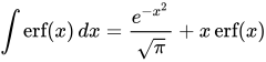
Not all closed-form expressions have closed-form antiderivatives; this study forms the subject of differential Galois theory, which was initially developed by Joseph Liouville in the 1830s and 1840s, leading to Liouville's theorem which classifies which expressions have closed-form antiderivatives. A simple example of a function without a closed-form antiderivative is e−x2, whose antiderivative is (up to constants) the error function.
Since 1968 there is the Risch algorithm for determining indefinite integrals that can be expressed in term of elementary functions, typically using a computer algebra system. Integrals that cannot be expressed using elementary functions can be manipulated symbolically using general functions such as the Meijer G-function.
Lists of integrals
[edit]More detail may be found on the following pages for the lists of integrals:
- List of integrals of rational functions
- List of integrals of irrational algebraic functions
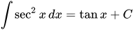
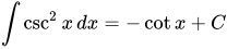
- List of integrals of trigonometric functions
- List of integrals of inverse trigonometric functions
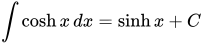
- List of integrals of hyperbolic functions
- List of integrals of inverse hyperbolic functions
- List of integrals of exponential functions
- List of integrals of logarithmic functions
- List of integrals of Gaussian functions
Gradshteyn, Ryzhik, Geronimus, Tseytlin, Jeffrey, Zwillinger, and Moll's (GR) Table of Integrals, Series, and Products contains a large collection of results. An even larger, multivolume table is the Integrals and Series by Prudnikov, Brychkov, and Marichev (with volumes 1–3 listing integrals and series of elementary and special functions, volume 4–5 are tables of Laplace transforms). More compact collections can be found in e.g. Brychkov, Marichev, Prudnikov's Tables of Indefinite Integrals, or as chapters in Zwillinger's CRC Standard Mathematical Tables and Formulae or Bronshtein and Semendyayev's Guide Book to Mathematics, Handbook of Mathematics or Users' Guide to Mathematics, and other mathematical handbooks.
Other useful resources include Abramowitz and Stegun and the Bateman Manuscript Project. Both works contain many identities concerning specific integrals, which are organized with the most relevant topic instead of being collected into a separate table. Two volumes of the Bateman Manuscript are specific to integral transforms.
There are several web sites which have tables of integrals and integrals on demand. Wolfram Alpha can show results, and for some simpler expressions, also the intermediate steps of the integration. Wolfram Research also operates another online service, the Mathematica Online Integrator.
Integrals of simple functions
[edit]C is used for an arbitrary constant of integration that can only be determined if something about the value of the integral at some point is known. Thus, each function has an infinite number of antiderivatives.
These formulas only state in another form the assertions in the table of derivatives.
Integrals with a singularity
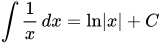
[edit]When there is a singularity in the function being integrated such that the antiderivative becomes undefined at some point (the singularity), then C does not need to be the same on both sides of the singularity. The forms below normally assume the Cauchy principal value around a singularity in the value of C, but this is not necessary in general. For instance, in there is a singularity at 0 and the antiderivative becomes infinite there. If the integral above were to be used to compute a definite integral between −1 and 1, one would get the wrong answer 0. This however is the Cauchy principal value of the integral around the singularity. If the integration is done in the complex plane the result depends on the path around the origin, in this case the singularity contributes −iπ when using a path above the origin and iπ for a path below the origin. A function on the real line could use a completely different value of C on either side of the origin as in:[2]

Rational functions
[edit]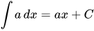
The following function has a non-integrable singularity at 0 for n ≤ −1:
- (Cavalieri's quadrature formula)
-
- More generally,[3]




Exponential functions
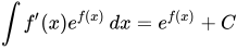
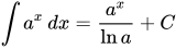
[edit]- (if is a positive integer)
- (if is a positive integer)




Logarithms
[edit]

Trigonometric functions
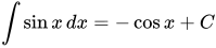
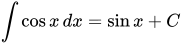
[edit]-
- (See Integral of the secant function. This result was a well-known conjecture in the 17th century.)
-
- (See integral of secant cubed.)








Inverse trigonometric functions
[edit]





Hyperbolic functions
[edit]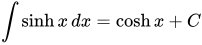



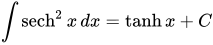



Inverse hyperbolic functions
[edit]





Products of functions proportional to their second derivatives
[edit]



Absolute-value functions
[edit]Let f be a continuous function, that has at most one zero. If f has a zero, let g be the unique antiderivative of f that is zero at the root of f; otherwise, let g be any antiderivative of f. Then where sgn(x) is the sign function, which takes the values −1, 0, 1 when x is respectively negative, zero or positive.

This can be proved by computing the derivative of the right-hand side of the formula, taking into account that the condition on g is here for insuring the continuity of the integral.
This gives the following formulas (where a ≠ 0), which are valid over any interval where f is continuous (over larger intervals, the constant C must be replaced by a piecewise constant function):
- when n is odd, and .
- when for some integer n.
- when for some integer n.
- when for some integer n.
- when for some integer n.








If the function f does not have any continuous antiderivative which takes the value zero at the zeros of f (this is the case for the sine and the cosine functions), then sgn(f(x)) ∫ f(x) dx is an antiderivative of f on every interval on which f is not zero, but may be discontinuous at the points where f(x) = 0. For having a continuous antiderivative, one has thus to add a well chosen step function. If we also use the fact that the absolute values of sine and cosine are periodic with period π, then we get:


Special functions
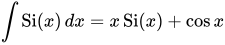
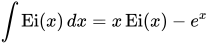
[edit]Ci, Si: Trigonometric integrals, Ei: Exponential integral, li: Logarithmic integral function, erf: Error function



Definite integrals lacking closed-form antiderivatives
[edit]There are some functions whose antiderivatives cannot be expressed in closed form. However, the values of the definite integrals of some of these functions over some common intervals can be calculated. A few useful integrals are given below.
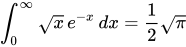
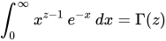
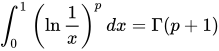
- (see also Gamma function)
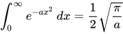
- for a > 0 (the Gaussian integral)
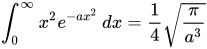
- for a > 0
- for a > 0, n is a positive integer and !! is the double factorial.
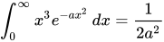
- when a > 0
- for a > 0, n = 0, 1, 2, ....
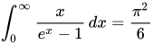
- (see also Bernoulli number)
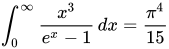
- (used in the derivation of Planck's law in physics)
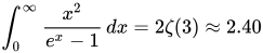
- for (see also Riemann zeta function)
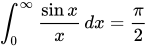
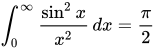
- (see sinc function and the Dirichlet integral)
- (if n is a positive integer and !! is the double factorial).
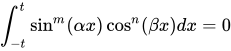
- (for α, β, m, n integers with β ≠ 0 and m, n ≥ 0, see also Binomial coefficient)
- (for α, β real, n a non-negative integer, and m an odd, positive integer; since the integrand is odd)
- (for α, β, m, n integers with β ≠ 0 and m, n ≥ 0, see also Binomial coefficient)
- (for α, β, m, n integers with β ≠ 0 and m, n ≥ 0, see also Binomial coefficient)
- (where exp[u] is the exponential function eu, and a > 0.)
- (where is the Gamma function)
- (for Re(α) > 0 and Re(β) > 0, see Beta function)
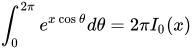
- (where I0(x) is the modified Bessel function of the first kind)
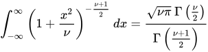
- (for ν > 0 , this is related to the probability density function of Student's t-distribution)









![{\displaystyle \int _{-\infty }^{\infty }e^{-(ax^{2}+bx+c)}\,dx={\sqrt {\frac {\pi }{a}}}\exp \left[{\frac {b^{2}-4ac}{4a}}\right]}](https://wikimedia.org/api/rest_v1/media/math/render/svg/9aac3de5d20ec70a35c8d52bafaa6a82c148b566)



If the function f has bounded variation on the interval [a,b], then the method of exhaustion provides a formula for the integral:

The "sophomore's dream": attributed to Johann Bernoulli.
![{\displaystyle {\begin{aligned}\int _{0}^{1}x^{-x}\,dx&=\sum _{n=1}^{\infty }n^{-n}&&(=1.29128\,59970\,6266\dots )\\[6pt]\int _{0}^{1}x^{x}\,dx&=-\sum _{n=1}^{\infty }(-n)^{-n}&&(=0.78343\,05107\,1213\dots )\end{aligned}}}](https://wikimedia.org/api/rest_v1/media/math/render/svg/3eb1c1f34b4606f5ebf9e88ecdb80a7681b8fcce)
See also
[edit]- Differentiation rules – Rules for computing derivatives of functions
- Incomplete gamma function – Types of special mathematical functions
- Indefinite sum – Inverse of a finite difference
- Integration using Euler's formula – Use of complex numbers to evaluate integrals
- Liouville's theorem (differential algebra) – Says when antiderivatives of elementary functions can be expressed as elementary functions
- List of limits
- List of mathematical identities
- List of mathematical series
- Nonelementary integral – Integrals not expressible in closed-form from elementary functions
- Symbolic integration – Computation of an antiderivatives
References
[edit]- ^ Hirsch, Meyer (1810). Integraltafeln: oder, Sammlung von integralformeln (in German). Duncker & Humblot.
- ^ Serge Lang . A First Course in Calculus, 5th edition, p. 290
- ^ "Reader Survey: log|x| + C", Tom Leinster, The n-category Café, March 19, 2012
Further reading
[edit]- Abramowitz, Milton; Stegun, Irene Ann, eds. (1983) [June 1964]. Handbook of Mathematical Functions with Formulas, Graphs, and Mathematical Tables. Applied Mathematics Series. Vol. 55 (Ninth reprint with additional corrections of tenth original printing with corrections (December 1972); first ed.). Washington D.C.; New York: United States Department of Commerce, National Bureau of Standards; Dover Publications. ISBN 978-0-486-61272-0. LCCN 64-60036. MR 0167642. LCCN 65-12253.
- Bronstein, Ilja Nikolaevič; Semendjajew, Konstantin Adolfovič (1987) [1945]. Grosche, Günter; Ziegler, Viktor; Ziegler, Dorothea (eds.). Taschenbuch der Mathematik (in German). Vol. 1. Translated by Ziegler, Viktor. Weiß, Jürgen (23 ed.). Thun and Frankfurt am Main: Verlag Harri Deutsch (and B. G. Teubner Verlagsgesellschaft, Leipzig). ISBN 3-87144-492-8.
- Gradshteyn, Izrail Solomonovich; Ryzhik, Iosif Moiseevich; Geronimus, Yuri Veniaminovich; Tseytlin, Michail Yulyevich; Jeffrey, Alan (2015) [October 2014]. Zwillinger, Daniel; Moll, Victor Hugo (eds.). Table of Integrals, Series, and Products. Translated by Scripta Technica, Inc. (8 ed.). Academic Press, Inc. ISBN 978-0-12-384933-5. LCCN 2014010276. (Several previous editions as well.)
- Prudnikov, Anatolii Platonovich (Прудников, Анатолий Платонович); Brychkov, Yuri A. (Брычков, Ю. А.); Marichev, Oleg Igorevich (Маричев, Олег Игоревич) (1988–1992) [1981−1986 (Russian)]. Integrals and Series. Vol. 1–5. Translated by Queen, N. M. (1 ed.). (Nauka) Gordon & Breach Science Publishers/CRC Press. ISBN 2-88124-097-6.
{{cite book}}: CS1 maint: multiple names: authors list (link). Second revised edition (Russian), volume 1–3, Fiziko-Matematicheskaya Literatura, 2003. - Yuri A. Brychkov (Ю. А. Брычков), Handbook of Special Functions: Derivatives, Integrals, Series and Other Formulas. Russian edition, Fiziko-Matematicheskaya Literatura, 2006. English edition, Chapman & Hall/CRC Press, 2008, ISBN 1-58488-956-X / 9781584889564.
- Daniel Zwillinger. CRC Standard Mathematical Tables and Formulae, 31st edition. Chapman & Hall/CRC Press, 2002. ISBN 1-58488-291-3. (Many earlier editions as well.)
- Meyer Hirsch, Integraltafeln oder Sammlung von Integralformeln (Duncker und Humblot, Berlin, 1810)
- Meyer Hirsch, Integral Tables Or A Collection of Integral Formulae (Baynes and son, London, 1823) [English translation of Integraltafeln]
- David Bierens de Haan, Nouvelles Tables d'Intégrales définies (Engels, Leiden, 1862)
- Benjamin O. Pierce A short table of integrals - revised edition (Ginn & co., Boston, 1899)
External links
[edit]Tables of integrals
[edit]- Paul's Online Math Notes
- A. Dieckmann, Table of Integrals (Elliptic Functions, Square Roots, Inverse Tangents and More Exotic Functions): Indefinite Integrals Definite Integrals
- Math Major: A Table of Integrals
- O'Brien, Francis J. Jr. "500 Integrals of Elementary and Special Functions". Derived integrals of exponential, logarithmic functions and special functions.
- Rule-based Integration Precisely defined indefinite integration rules covering a wide class of integrands
- Mathar, Richard J. (2012). "Yet another table of integrals". arXiv:1207.5845 [math.CA].
Derivations
[edit]Online service
[edit]Open source programs
[edit]Videos
[edit]- The Single Most Overpowered Integration Technique in Existence. YouTube Video by Flammable Maths on symmetries


Lists of integrals
View on GrokipediaIntroduction to Integration
Definition and Fundamental Concepts
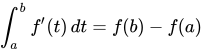
The indefinite integral of a function $ f(x) $, denoted by $ \int f(x) , dx $, represents the set of all antiderivatives of $ f(x) $. An antiderivative $ F(x) $ satisfies the condition $ F'(x) = f(x) $, and due to the constant nature of differentiation, the general solution includes an arbitrary constant of integration $ C $, yielding $ \int f(x) , dx = F(x) + C $. This formulation captures the family of functions whose derivatives recover the original integrand.[5] In contrast, the definite integral $ \int_a^b f(x) , dx $ quantifies the net accumulation of $ f(x) $ over the interval from $ a $ to $ b $, interpreted geometrically as the signed area between the curve $ y = f(x) $ and the x-axis. It arises as the limit of Riemann sums, where the interval is partitioned into subintervals, and the sum of areas of approximating rectangles (with heights given by function values at partition points) converges to the integral as the subinterval widths approach zero. The Fundamental Theorem of Calculus links this to antiderivatives, stating that if $ F(x) $ is an antiderivative of $ f(x) $, then $ \int_a^b f(x) , dx = F(b) - F(a) $.[6] Integrals play a central role in mathematics by inverting differentiation, enabling the solution of differential equations that model rates of change. In practical applications, such as physics, they facilitate computations like determining position from velocity via $ \int v(t) , dt = s(t) + C $, where $ s(t) $ is displacement, thus addressing problems of accumulation in fields ranging from engineering to economics.[7] A fundamental example illustrates these concepts through the power rule: for $ n \neq -1 $, the indefinite integral is $ \int x^n , dx = \frac{x^{n+1}}{n+1} + C $, which can be verified by differentiation.[8]Notation and Basic Properties
In lists of integrals, the standard notation for the indefinite integral of a function with respect to the variable is , which denotes the family of antiderivatives of . This Leibniz notation emphasizes the differential as an infinitesimal increment, facilitating techniques like substitution and parts. In contrast, Lagrange notation for antiderivatives is less common for integrals but may appear as where using prime notation for differentiation. For definite integrals, the notation specifies the limits of integration from (lower) to (upper), yielding a numerical value that represents the signed area under the curve of over that interval.[9] A fundamental property of integrals is linearity, which allows the operation to distribute over addition and scalar multiplication. Specifically, for constants and , and integrable functions and ,Historical Development
Ancient and Pre-Calculus Contributions
Early contributions to the computation of areas and summations, precursors to integral calculus, emerged in ancient civilizations through geometric and algebraic methods focused on specific problems rather than general theories. In ancient Greece, Archimedes of Syracuse (c. 287–212 BCE) employed the method of exhaustion to determine the area of a parabolic segment in his work Quadrature of the Parabola (c. 250 BCE). This technique involved inscribing a sequence of polygons within the segment, with each subsequent polygon adding triangles whose areas formed a geometric series summing to four-thirds the area of the initial inscribed triangle, effectively computing the area of a parabolic segment as four-thirds the area of the initial inscribed triangle, corresponding to the modern integral of a quadratic function such as (with appropriate scaling), without invoking limits or infinitesimals.[14] Similarly, Archimedes applied exhaustion to circle quadrature in Measurement of a Circle (c. 250 BCE), bounding the circle's area between inscribed and circumscribed polygons to establish it as equal to , where was approximated between 3 10/71 and 3 1/7, enabling precise computations of circular areas.[15] In ancient India, mathematicians developed summation techniques that facilitated area-related calculations, particularly in astronomy and geometry. Aryabhata (476–550 CE) provided explicit formulas in Aryabhatiya (499 CE) for the sums of powers of natural numbers, such as the sum of first naturals , sum of squares , and sum of cubes , which underpinned approximations for areas under polynomial curves and trigonometric functions like sine.[16] His construction of the first sine table, using second-order finite differences on a circle of radius approximately 3438 arcminutes, allowed for interpolations that approximated integrals involving sine, such as those in planetary motion models, though without a formal integral concept. These algebraic tools, combined with geometric approximations like Aryabhata's , supported specific quadratures in calendrical and architectural contexts.[16] By the early modern period, methods bridging geometry and summation appeared in Europe. Bonaventura Cavalieri (1598–1647) introduced the method of indivisibles in Geometria indivisibilibus continuorum nova quadam ratione promota (1635), treating plane figures as aggregates of "all the lines" (indivisible line segments) parallel to a base, whose lengths sum to the area. This approach, a precursor to Riemann sums, compared figures by the ratios of their indivisible collections—for instance, showing the area under a linear function equals half the rectangle's area—without relying on infinitesimals, instead using magnitude comparisons rooted in ancient Greek traditions.[17] Collectively, these pre-calculus techniques enabled targeted area and volume computations, such as parabolic segments and circle quadratures, but lacked the general antiderivative framework that would define formal integration.[14]Formalization in Calculus
The formalization of integration within calculus began in the late 17th century, when Isaac Newton and Gottfried Wilhelm Leibniz independently developed the foundational concepts of the discipline. Newton formulated his method of fluxions during the years 1665–1667, viewing integration as the inverse process of differentiation to find areas under curves, though his Method of Fluxions treatise, completed around 1671, was not published until posthumously in 1736; he employed related ideas in geometric form in his Philosophiæ Naturalis Principia Mathematica (1687). Leibniz, working in the 1670s, emphasized infinitesimals and introduced the integral symbol ∫ in an unpublished manuscript dated October 29, 1675, denoting the "sum" of infinitesimal quantities, a notation that persists today. These innovations transformed integration from ad hoc geometric techniques into a systematic analytical tool, enabling the computation of antiderivatives for a growing array of functions.[18][19] In the 18th century, Leonhard Euler advanced this framework through extensive systematic studies, culminating in his three-volume Institutiones calculi integralis published between 1768 and 1770. Euler explored integrals expressible in terms of elementary functions, deriving numerous formulas and employing series expansions, particularly trigonometric series, to evaluate complex forms that eluded earlier methods. His work not only enriched the repertoire of known integrals but also established methods for their classification and computation, setting the stage for compiled tables by demonstrating the breadth of integrable expressions. Euler's contributions, grounded in the Leibnizian notation, facilitated practical applications in physics and astronomy.[20] The early 19th century saw the emergence of the first comprehensive tables of integrals, with Meyer Hirsch's Integraltafeln (1810) compiling over 200 formulas for indefinite integrals, serving as a key reference for researchers. This collection organized results from prior developments, making integration techniques more accessible. Concurrently, the rigorization of definite integrals progressed through the efforts of Augustin-Louis Cauchy and Bernhard Riemann. In his 1821 Cours d'analyse, Cauchy defined the definite integral as the limit of sums of Riemann-like partitions for continuous functions, providing an epsilon-delta foundation that eliminated reliance on infinitesimals. Riemann extended this in 1854 by generalizing the integral to bounded functions with discontinuities, using upper and lower sums to ensure convergence under milder conditions. These advancements ensured that lists of integrals rested on a solid theoretical base, influencing subsequent tabular compilations.Structure of Integral Lists
Organization Principles
Lists of integrals are primarily organized by categorizing the integrands according to their function types, separating elementary functions—such as polynomials, rational expressions, exponentials, logarithms, trigonometric, and hyperbolic functions—from special functions like Bessel, gamma, and error functions.[21] This approach facilitates targeted reference, allowing users to locate relevant formulas based on the mathematical structure involved.[22] In comprehensive compilations, such as the Gradshteyn and Ryzhik tables, further subdivision occurs by the specific form of the integrand within each category, grouping similar expressions for systematic access. The ordering of entries within these categories typically follows a thematic structure, progressing from simpler to more complex forms. Reduction formulas are systematically included, particularly for powers of functions, enabling recursive computation; for instance, the reduction formula for allows evaluation of higher-order trigonometric integrals from lower ones. This inclusion ensures that lists address iterative patterns common in applications. Indefinite integrals are presented with the arbitrary constant , while definite integrals specify limits and any associated conditions.[21] Domains of validity and convergence criteria are explicitly noted, especially for integrals prone to issues like logarithmic singularities, where absolute convergence or branch cuts must be considered to avoid invalid applications. To achieve completeness without exhaustive enumeration, lists incorporate principles that account for derivable forms through standard techniques, including common substitutions (e.g., ) and identities such as trigonometric-to-exponential conversions via Euler's formula. This strategy emphasizes core patterns, assuming users can adapt entries via algebraic manipulation for related cases.Common Formats and Resources
Lists of integrals are commonly presented in tabular formats within printed handbooks, where formulas are organized by function type and listed alongside their antiderivatives, often with conditions for validity. A seminal example is the multi-volume Table of Integrals, Series, and Products by I.S. Gradshteyn and I.M. Ryzhik, first published in 1943 and continually expanded through subsequent editions, providing over 10,000 entries in a structured tabular layout.[23] Another influential printed resource is the Handbook of Elliptic Integrals for Engineers and Physicists by P.F. Byrd and M.D. Friedman, published in 1954, which tabulates elliptic integrals and related transformations in a concise, application-oriented format.[24] The eighth edition of Gradshteyn and Ryzhik, edited by Daniel Zwillinger in 2014, maintains this tabular tradition while incorporating 25% new material and corrections.[23] In contrast, online databases offer interactive and searchable formats that surpass traditional tables by allowing users to input specific integrals for computation or lookup. Wolfram Alpha provides an interactive query system for indefinite and definite integrals, leveraging computational algorithms to generate step-by-step solutions and verify results.[25] The NIST Digital Library of Mathematical Functions (DLMF) serves as a comprehensive digital repository, featuring verified formulas for integrals involving special functions, with hyperlinks to derivations and numerical evaluations.[26] Modern integral lists frequently incorporate software-verified formulas to enhance accuracy, addressing omissions and errors prevalent in older tables, such as those from the 19th century where computational limitations led to uncorrected inaccuracies in published works.[27] For instance, recent editions of established handbooks systematically revise entries based on computational checks, ensuring reliability for contemporary applications.[23]Indefinite Integrals of Elementary Functions
Polynomials and Rational Functions
The integration of polynomials relies on the power rule, which states that for a real number $ n \neq -1 $, the antiderivative of $ x^n $ is $ \frac{x^{n+1}}{n+1} + C $, where $ C $ is the constant of integration.[28] This rule is derived by reversing the differentiation process and applies directly to monomials, allowing the integration of any polynomial by summing the antiderivatives of its terms.[29] For instance, the integral of a linear polynomial $ ax + b $ is computed term by term as $ \frac{a}{2}x^2 + bx + C $.[30] When $ n = -1 $, the power rule does not apply, and instead $ \int \frac{1}{x} , dx = \ln |x| + C $, which is a foundational result for rational functions involving this form.[29] Polynomials of higher degree follow the same principle; for example, $ \int x^3 , dx = \frac{x^4}{4} + C $.[28] Rational functions, which are ratios of polynomials, require decomposition into partial fractions before integration when the degree of the numerator is less than the degree of the denominator.[31] This method expresses the rational function as a sum of simpler fractions, each integrable using the power rule or logarithmic forms.[32] For a proper rational function with distinct linear factors in the denominator, the partial fraction decomposition takes the form $ \frac{P(x)}{Q(x)} = \sum \frac{A_i}{x - r_i} $, where $ r_i $ are the roots and $ A_i $ are constants found by solving a system of equations.[33] A classic example is $ \int \frac{1}{x^2 - 1} , dx $, where $ x^2 - 1 = (x-1)(x+1) $, decomposing to $ \frac{1}{x^2 - 1} = \frac{1/2}{x-1} - \frac{1/2}{x+1} $, yielding $ \frac{1}{2} \ln \left| \frac{x-1}{x+1} \right| + C $.[31] For repeated factors or irreducible quadratics, the decomposition includes additional terms like $ \frac{A}{(x-r)^k} $ or $ \frac{Bx + C}{x^2 + px + q} $, integrated accordingly.[34] Indefinite integrals of power functions with exponents between -1 and 0 require domain restrictions due to singularities; for example, $ \int x^{-1/2} , dx = 2x^{1/2} + C $ for $ x > 0 $.[28] This ensures the antiderivative remains defined in the appropriate interval, avoiding singularities at zero or negative values.[29]Exponential and Logarithmic Functions
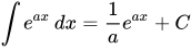
The integrals of exponential and logarithmic functions form a core component of lists of indefinite integrals, as these functions model continuous growth and decay processes in mathematics and applications such as population dynamics and radioactive decay. The antiderivative of the basic exponential function is straightforward due to its self-derivative property, while logarithmic integrals often require integration by parts to resolve. These results extend to composite forms through substitution or parts, enabling evaluation of more complex expressions without resorting to special functions. The integral for follows directly from the chain rule in reverse, as the derivative of is . This generalizes to via the substitution , , which transforms the integral into before back-substituting. For example, this substitution applies to integrals like , yielding $ \frac{1}{2} e^{x^2} + C $. For exponential functions with base , , the integral is , derived by rewriting and applying the previous result with the constant . This form highlights the role of the natural logarithm in unifying different bases. The natural logarithm integral is obtained using integration by parts, setting , so , , yielding . Common composite integrals include , found via integration by parts with , so , , giving . Similarly, uses substitution , , reducing to .Trigonometric and Inverse Trigonometric Functions
The integrals of basic trigonometric functions form a foundational set in calculus, enabling the evaluation of antiderivatives for periodic functions encountered in physics, engineering, and signal processing. These integrals are typically derived using differentiation rules in reverse or substitution techniques, and they appear in standard tables for quick reference. For instance, the integral of the sine function with a linear argument is a core example, generalizing the unit case to handle scaled frequencies. The antiderivative of is given byHyperbolic and Inverse Hyperbolic Functions
Hyperbolic functions arise naturally from exponential expressions and play a key role in differential equations and physical models, such as the catenary curve describing a hanging chain. Their antiderivatives are typically elementary and follow patterns similar to trigonometric integrals, though without periodicity. These integrals can often be derived using substitution or by leveraging the exponential definitions of hyperbolic functions, which connect them to logarithmic forms.[40] The basic indefinite integrals for the hyperbolic sine and cosine functions are straightforward, reflecting their roles as mutual derivatives up to scaling. For a constant ,Indefinite Integrals Involving Special Cases
Singularities and Absolute Values
Integrals involving absolute values and singularities often require piecewise definitions or special techniques due to discontinuities or non-differentiability at specific points, such as x = 0. The absolute value function |x| introduces a non-differentiable point at the origin, leading to an antiderivative that combines linear and quadratic terms. The indefinite integral is given byProducts Related to Derivatives
Integrals of products involving a function and its derivatives often arise when applying integration by parts to expressions like , where is the second derivative of . This technique, derived from the product rule for differentiation, transforms the integral into a boundary term minus another integral. Specifically, setting and yields and , resulting in the identity .[12] This relation is particularly useful for simple functions where the remaining integral can be evaluated elementarily. For concrete examples, consider trigonometric functions. The integral corresponds to the case where and . This evaluates to , using the power-reduction formula for .[44] Similarly, for exponential forms related to Gaussian derivatives, . Here, the integrand is proportional to the derivative of , since , allowing direct evaluation by substitution , .[44] Such products are emphasized in integral tables for cases where closed forms are achievable, particularly polynomials multiplied by exponentials or trigonometric functions, as these often reduce via substitution or repeated integration by parts. These integrals frequently appear in variational problems, where functionals like are extremized; integration by parts then derives the Euler-Lagrange equations, such as for the simplest quadratic case, linking the product forms to physical principles like least action.[45] Standard tables prioritize these solvable instances to aid computations in applied contexts, avoiding more complex non-elementary outcomes.Error Functions and Other Special Integrals
The error function and related special integrals arise in contexts where elementary antiderivatives are unavailable, such as the Gaussian integral, leading to transcendental functions essential in probability, heat conduction, and diffusion processes.[46] These functions are defined through definite integrals but serve as antiderivatives for indefinite forms, providing closed-form expressions where direct integration fails.[46] The error function, denoted , is defined asDefinite Integrals and Closed-Form Challenges
Standard Definite Integrals with Closed Forms
Standard definite integrals with closed forms refer to those improper integrals involving elementary functions over infinite or semi-infinite intervals that evaluate to exact expressions without requiring special functions beyond basic constants and gamma functions for generalization. These integrals often arise in probability, physics, and analysis, providing foundational results for more complex evaluations. Key examples include the Gaussian integral, the exponential decay integral, the Wallis integrals for powers of sine, certain logarithmic integrals derived via series expansions, the Dirichlet integral, and Legendre integrals expressed via the beta function. The Gaussian integral is a cornerstone result, given byDefinite Integrals Lacking Closed Forms
Definite integrals lacking closed forms are those whose values cannot be expressed in terms of elementary functions alone, often requiring special functions beyond gamma and beta, infinite series, or advanced techniques such as contour integration for evaluation. These integrals arise frequently in mathematical analysis and applications, where their definite values provide important constants or relations, even if the corresponding antiderivatives remain non-elementary. Lists of such integrals typically emphasize their evaluation methods and numerical approximations, highlighting the need for non-standard approaches like residue theorem or series expansions.[52] One prominent example is Sophomore's dream, which consists of the pair of identitiesAdvanced and Applied Integral Lists
Integrals in Complex Analysis
In complex analysis, contour integrals over closed paths in the complex plane provide a framework for evaluating integrals of analytic functions, leveraging their singularities through residues. These methods are essential for lists of integrals involving poles and essential singularities, extending beyond real-line computations by exploiting the geometry of the complex domain. Key theorems like Cauchy's integral formula and the residue theorem form the basis for such evaluations, allowing systematic computation of residues for common function classes such as rational and trigonometric expressions.[53] Cauchy's integral formula states that if is analytic inside and on a simple closed positively oriented contour , and is a point inside , then- For , poles at ; , .
- For , simple pole at with residue where and ; order-2 pole at with residue .