

Stochastic process
View on Wikipedia| Part of a series on statistics |
| Probability theory |
|---|
 |

In probability theory and related fields, a stochastic (/stəˈkæstɪk/) or random process is a mathematical object usually defined as a family of random variables in a probability space, where the index of the family often has the interpretation of time. Stochastic processes are widely used as mathematical models of systems and phenomena that appear to vary in a random manner. Examples include the growth of a bacterial population, an electrical current fluctuating due to thermal noise, or the movement of a gas molecule.[1][4][5] Stochastic processes have applications in many disciplines such as biology,[6] chemistry,[7] ecology,[8] neuroscience,[9] physics,[10] image processing, signal processing,[11] control theory,[12] information theory,[13] computer science,[14] and telecommunications.[15] Furthermore, seemingly random changes in financial markets have motivated the extensive use of stochastic processes in finance.[16][17][18]
Applications and the study of phenomena have in turn inspired the proposal of new stochastic processes. Examples of such stochastic processes include the Wiener process or Brownian motion process,[a] used by Louis Bachelier to study price changes on the Paris Bourse,[21] and the Poisson process, used by A. K. Erlang to study the number of phone calls occurring in a certain period of time.[22] These two stochastic processes are considered the most important and central in the theory of stochastic processes,[1][4][23] and were invented repeatedly and independently, both before and after Bachelier and Erlang, in different settings and countries.[21][24]
The term random function is also used to refer to a stochastic or random process,[25][26] because a stochastic process can also be interpreted as a random element in a function space.[27][28] The terms stochastic process and random process are used interchangeably, often with no specific mathematical space for the set that indexes the random variables.[27][29] But often these two terms are used when the random variables are indexed by the integers or an interval of the real line.[5][29] If the random variables are indexed by the Cartesian plane or some higher-dimensional Euclidean space, then the collection of random variables is usually called a random field instead.[5][30] The values of a stochastic process are not always numbers and can be vectors or other mathematical objects.[5][28]
Based on their mathematical properties, stochastic processes can be grouped into various categories, which include random walks,[31] martingales,[32] Markov processes,[33] Lévy processes,[34] Gaussian processes,[35] random fields,[36] renewal processes, and branching processes.[37] The study of stochastic processes uses mathematical knowledge and techniques from probability, calculus, linear algebra, set theory, and topology[38][39][40] as well as branches of mathematical analysis such as real analysis, measure theory, Fourier analysis, and functional analysis.[41][42][43] The theory of stochastic processes is considered to be an important contribution to mathematics[44] and it continues to be an active topic of research for both theoretical reasons and applications.[45][46][47]
Introduction
[edit]A stochastic or random process can be defined as a collection of random variables that is indexed by some mathematical set, meaning that each random variable of the stochastic process is uniquely associated with an element in the set.[4][5] The set used to index the random variables is called the index set. Historically, the index set was some subset of the real line, such as the natural numbers, giving the index set the interpretation of time.[1] Each random variable in the collection takes values from the same mathematical space known as the state space. This state space can be, for example, the integers, the real line or -dimensional Euclidean space.[1][5] An increment is the amount that a stochastic process changes between two index values, often interpreted as two points in time.[48][49] A stochastic process can have many outcomes, due to its randomness, and a single outcome of a stochastic process is called, among other names, a sample function or realization.[28][50]


Classifications
[edit]A stochastic process can be classified in different ways, for example, by its state space, its index set, or the dependence among the random variables. One common way of classification is by the cardinality of the index set and the state space.[51][52][53]
When interpreted as time, if the index set of a stochastic process has a finite or countable number of elements, such as a finite set of numbers, the set of integers, or the natural numbers, then the stochastic process is said to be in discrete time.[54][55] If the index set is some interval of the real line, then time is said to be continuous. The two types of stochastic processes are respectively referred to as discrete-time and continuous-time stochastic processes.[48][56][57] Discrete-time stochastic processes are considered easier to study because continuous-time processes require more advanced mathematical techniques and knowledge, particularly due to the index set being uncountable.[58][59] If the index set is the integers, or some subset of them, then the stochastic process can also be called a random sequence.[55]
If the state space is the integers or natural numbers, then the stochastic process is called a discrete or integer-valued stochastic process. If the state space is the real line, then the stochastic process is referred to as a real-valued stochastic process or a process with continuous state space. If the state space is -dimensional Euclidean space, then the stochastic process is called a -dimensional vector process or -vector process.[51][52]
Etymology
[edit]The word stochastic in English was originally used as an adjective with the definition "pertaining to conjecturing", and stemming from a Greek word meaning "to aim at a mark, guess", and the Oxford English Dictionary gives the year 1662 as its earliest occurrence.[60] In his work on probability Ars Conjectandi, originally published in Latin in 1713, Jakob Bernoulli used the phrase "Ars Conjectandi sive Stochastice", which has been translated to "the art of conjecturing or stochastics".[61] This phrase was used, with reference to Bernoulli, by Ladislaus Bortkiewicz[62] who in 1917 wrote in German the word stochastik with a sense meaning random. The term stochastic process first appeared in English in a 1934 paper by Joseph Doob.[60] For the term and a specific mathematical definition, Doob cited another 1934 paper, where the term stochastischer Prozeß was used in German by Aleksandr Khinchin,[63][64] though the German term had been used earlier, for example, by Andrei Kolmogorov in 1931.[65]
According to the Oxford English Dictionary, early occurrences of the word random in English with its current meaning, which relates to chance or luck, date back to the 16th century, while earlier recorded usages started in the 14th century as a noun meaning "impetuosity, great speed, force, or violence (in riding, running, striking, etc.)". The word itself comes from a Middle French word meaning "speed, haste", and it is probably derived from a French verb meaning "to run" or "to gallop". The first written appearance of the term random process pre-dates stochastic process, which the Oxford English Dictionary also gives as a synonym, and was used in an article by Francis Edgeworth published in 1888.[66]
Terminology
[edit]The definition of a stochastic process varies,[67] but a stochastic process is traditionally defined as a collection of random variables indexed by some set.[68][69] The terms random process and stochastic process are considered synonyms and are used interchangeably, without the index set being precisely specified.[27][29][30][70][71][72] Both "collection",[28][70] or "family" are used[4][73] while instead of "index set", sometimes the terms "parameter set"[28] or "parameter space"[30] are used.
The term random function is also used to refer to a stochastic or random process,[5][74][75] though sometimes it is only used when the stochastic process takes real values.[28][73] This term is also used when the index sets are mathematical spaces other than the real line,[5][76] while the terms stochastic process and random process are usually used when the index set is interpreted as time,[5][76][77] and other terms are used such as random field when the index set is -dimensional Euclidean space or a manifold.[5][28][30]

Notation
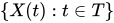
[edit]A stochastic process can be denoted, among other ways, by ,[56] ,[69] [78] or simply as . Some authors mistakenly write even though it is an abuse of function notation.[79] For example, or are used to refer to the random variable with the index , and not the entire stochastic process.[78] If the index set is , then one can write, for example, to denote the stochastic process.[29]


Examples
[edit]Bernoulli process
[edit]One of the simplest stochastic processes is the Bernoulli process,[80] which is a sequence of independent and identically distributed (iid) random variables, where each random variable takes either the value one or zero, say one with probability and zero with probability . This process can be linked to an idealisation of repeatedly flipping a coin, where the probability of obtaining a head is taken to be and its value is one, while the value of a tail is zero.[81] In other words, a Bernoulli process is a sequence of iid Bernoulli random variables,[82] where each idealised coin flip is an example of a Bernoulli trial.[83]


Random walk
[edit]Random walks are stochastic processes that are usually defined as sums of iid random variables or random vectors in Euclidean space, so they are processes that change in discrete time.[84][85][86][87][88] But some also use the term to refer to processes that change in continuous time,[89] particularly the Wiener process used in financial models, which has led to some confusion, resulting in its criticism.[90] There are various other types of random walks, defined so their state spaces can be other mathematical objects, such as lattices and groups, and in general they are highly studied and have many applications in different disciplines.[89][91]
A classic example of a random walk is known as the simple random walk, which is a stochastic process in discrete time with the integers as the state space, and is based on a Bernoulli process, where each Bernoulli variable takes either the value positive one or negative one. In other words, the simple random walk takes place on the integers, and its value increases by one with probability, say, , or decreases by one with probability , so the index set of this random walk is the natural numbers, while its state space is the integers. If , this random walk is called a symmetric random walk.[92][93]

Wiener process
[edit]The Wiener process is a stochastic process with stationary and independent increments that are normally distributed based on the size of the increments.[2][94] The Wiener process is named after Norbert Wiener, who proved its mathematical existence, but the process is also called the Brownian motion process or just Brownian motion due to its historical connection as a model for Brownian movement in liquids.[95][96][97]

Playing a central role in the theory of probability, the Wiener process is often considered the most important and studied stochastic process, with connections to other stochastic processes.[1][2][3][98][99][100][101] Its index set and state space are the non-negative numbers and real numbers, respectively, so it has both continuous index set and states space.[102] But the process can be defined more generally so its state space can be -dimensional Euclidean space.[91][99][103] If the mean of any increment is zero, then the resulting Wiener or Brownian motion process is said to have zero drift. If the mean of the increment for any two points in time is equal to the time difference multiplied by some constant , which is a real number, then the resulting stochastic process is said to have drift .[104][105][106]

Almost surely, a sample path of a Wiener process is continuous everywhere but nowhere differentiable. It can be considered as a continuous version of the simple random walk.[49][105] The process arises as the mathematical limit of other stochastic processes such as certain random walks rescaled,[107][108] which is the subject of Donsker's theorem or invariance principle, also known as the functional central limit theorem.[109][110][111]
The Wiener process is a member of some important families of stochastic processes, including Markov processes, Lévy processes and Gaussian processes.[2][49] The process also has many applications and is the main stochastic process used in stochastic calculus.[112][113] It plays a central role in quantitative finance,[114][115] where it is used, for example, in the Black–Scholes–Merton model.[116] The process is also used in different fields, including the majority of natural sciences as well as some branches of social sciences, as a mathematical model for various random phenomena.[3][117][118]
Poisson process
[edit]The Poisson process is a stochastic process that has different forms and definitions.[119][120] It can be defined as a counting process, which is a stochastic process that represents the random number of points or events up to some time. The number of points of the process that are located in the interval from zero to some given time is a Poisson random variable that depends on that time and some parameter. This process has the natural numbers as its state space and the non-negative numbers as its index set. This process is also called the Poisson counting process, since it can be interpreted as an example of a counting process.[119]
If a Poisson process is defined with a single positive constant, then the process is called a homogeneous Poisson process.[119][121] The homogeneous Poisson process is a member of important classes of stochastic processes such as Markov processes and Lévy processes.[49]
The homogeneous Poisson process can be defined and generalized in different ways. It can be defined such that its index set is the real line, and this stochastic process is also called the stationary Poisson process.[122][123] If the parameter constant of the Poisson process is replaced with some non-negative integrable function of , the resulting process is called an inhomogeneous or nonhomogeneous Poisson process, where the average density of points of the process is no longer constant.[124] Serving as a fundamental process in queueing theory, the Poisson process is an important process for mathematical models, where it finds applications for models of events randomly occurring in certain time windows.[125][126]
Defined on the real line, the Poisson process can be interpreted as a stochastic process,[49][127] among other random objects.[128][129] But then it can be defined on the -dimensional Euclidean space or other mathematical spaces,[130] where it is often interpreted as a random set or a random counting measure, instead of a stochastic process.[128][129] In this setting, the Poisson process, also called the Poisson point process, is one of the most important objects in probability theory, both for applications and theoretical reasons.[22][131] But it has been remarked that the Poisson process does not receive as much attention as it should, partly due to it often being considered just on the real line, and not on other mathematical spaces.[131][132]
Definitions
[edit]Stochastic process
[edit]A stochastic process is defined as a collection of random variables defined on a common probability space , where is a sample space, is a -algebra, and is a probability measure; and the random variables, indexed by some set , all take values in the same mathematical space , which must be measurable with respect to some -algebra .[28]


In other words, for a given probability space and a measurable space , a stochastic process is a collection of -valued random variables, which can be written as:[80]


Historically, in many problems from the natural sciences a point had the meaning of time, so is a random variable representing a value observed at time .[133] A stochastic process can also be written as to reflect that it is actually a function of two variables, and .[28][134]



There are other ways to consider a stochastic process, with the above definition being considered the traditional one.[68][69] For example, a stochastic process can be interpreted or defined as a -valued random variable, where is the space of all the possible functions from the set into the space .[27][68] However this alternative definition as a "function-valued random variable" in general requires additional regularity assumptions to be well-defined.[135]

Index set
[edit]The set is called the index set[4][51] or parameter set[28][136] of the stochastic process. Often this set is some subset of the real line, such as the natural numbers or an interval, giving the set the interpretation of time.[1] In addition to these sets, the index set can be another set with a total order or a more general set,[1][54] such as the Cartesian plane or -dimensional Euclidean space, where an element can represent a point in space.[48][137] That said, many results and theorems are only possible for stochastic processes with a totally ordered index set.[138]

State space
[edit]The mathematical space of a stochastic process is called its state space. This mathematical space can be defined using integers, real lines, -dimensional Euclidean spaces, complex planes, or more abstract mathematical spaces. The state space is defined using elements that reflect the different values that the stochastic process can take.[1][5][28][51][56]
Sample function
[edit]A sample function is a single outcome of a stochastic process, so it is formed by taking a single possible value of each random variable of the stochastic process.[28][139] More precisely, if is a stochastic process, then for any point , the mapping

is called a sample function, a realization, or, particularly when is interpreted as time, a sample path of the stochastic process .[50] This means that for a fixed , there exists a sample function that maps the index set to the state space .[28] Other names for a sample function of a stochastic process include trajectory, path function[140] or path.[141]
Increment
[edit]An increment of a stochastic process is the difference between two random variables of the same stochastic process. For a stochastic process with an index set that can be interpreted as time, an increment is how much the stochastic process changes over a certain time period. For example, if is a stochastic process with state space and index set , then for any two non-negative numbers and such that , the difference is a -valued random variable known as an increment.[48][49] When interested in the increments, often the state space is the real line or the natural numbers, but it can be -dimensional Euclidean space or more abstract spaces such as Banach spaces.[49]


Further definitions
[edit]Law
[edit]For a stochastic process defined on the probability space , the law of stochastic process is defined as the pushforward measure:

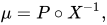
where is a probability measure, the symbol denotes function composition and is the pre-image of the measurable function or, equivalently, the -valued random variable , where is the space of all the possible -valued functions of , so the law of a stochastic process is a probability measure.[27][68][142][143]


For a measurable subset of , the pre-image of gives


so the law of a can be written as:[28]

The law of a stochastic process or a random variable is also called the probability law, probability distribution, or the distribution.[133][142][144][145][146]
Finite-dimensional probability distributions
[edit]For a stochastic process with law , its finite-dimensional distribution for is defined as:


This measure is the joint distribution of the random vector ; it can be viewed as a "projection" of the law onto a finite subset of .[27][147]


For any measurable subset of the -fold Cartesian power , the finite-dimensional distributions of a stochastic process can be written as:[28]



The finite-dimensional distributions of a stochastic process satisfy two mathematical conditions known as consistency conditions.[57]
Stationarity
[edit]Stationarity is a mathematical property that a stochastic process has when all the random variables of that stochastic process are identically distributed. In other words, if is a stationary stochastic process, then for any the random variable has the same distribution, which means that for any set of index set values , the corresponding random variables


all have the same probability distribution. The index set of a stationary stochastic process is usually interpreted as time, so it can be the integers or the real line.[148][149] But the concept of stationarity also exists for point processes and random fields, where the index set is not interpreted as time.[148][150][151]
When the index set can be interpreted as time, a stochastic process is said to be stationary if its finite-dimensional distributions are invariant under translations of time. This type of stochastic process can be used to describe a physical system that is in steady state, but still experiences random fluctuations.[148] The intuition behind stationarity is that as time passes the distribution of the stationary stochastic process remains the same.[152] A sequence of random variables forms a stationary stochastic process only if the random variables are identically distributed.[148]
A stochastic process with the above definition of stationarity is sometimes said to be strictly stationary, but there are other forms of stationarity. One example is when a discrete-time or continuous-time stochastic process is said to be stationary in the wide sense, then the process has a finite second moment for all and the covariance of the two random variables and depends only on the number for all .[152][153] Khinchin introduced the related concept of stationarity in the wide sense, which has other names including covariance stationarity or stationarity in the broad sense.[153][154]


Filtration
[edit]A filtration is an increasing sequence of sigma-algebras defined in relation to some probability space and an index set that has some total order relation, such as in the case of the index set being some subset of the real numbers. More formally, if a stochastic process has an index set with a total order, then a filtration , on a probability space is a family of sigma-algebras such that for all , where and denotes the total order of the index set .[51] With the concept of a filtration, it is possible to study the amount of information contained in a stochastic process at , which can be interpreted as time .[51][155] The intuition behind a filtration is that as time passes, more and more information on is known or available, which is captured in , resulting in finer and finer partitions of .[156][157]




Modification
[edit]A modification of a stochastic process is another stochastic process, which is closely related to the original stochastic process. More precisely, a stochastic process that has the same index set , state space , and probability space as another stochastic process is said to be a modification of if for all the following



holds. Two stochastic processes that are modifications of each other have the same finite-dimensional law[158] and they are said to be stochastically equivalent or equivalent.[159]
Instead of modification, the term version is also used,[150][160][161][162] however some authors use the term version when two stochastic processes have the same finite-dimensional distributions, but they may be defined on different probability spaces, so two processes that are modifications of each other, are also versions of each other, in the latter sense, but not the converse.[163][142]
If a continuous-time real-valued stochastic process meets certain moment conditions on its increments, then the Kolmogorov continuity theorem says that there exists a modification of this process that has continuous sample paths with probability one, so the stochastic process has a continuous modification or version.[161][162][164] The theorem can also be generalized to random fields so the index set is -dimensional Euclidean space[165] as well as to stochastic processes with metric spaces as their state spaces.[166]
Indistinguishable
[edit]Two stochastic processes and defined on the same probability space with the same index set and set space are said be indistinguishable if the following

holds.[142][158] If two and are modifications of each other and are almost surely continuous, then and are indistinguishable.[167]
Separability
[edit]Separability is a property of a stochastic process based on its index set in relation to the probability measure. The property is assumed so that functionals of stochastic processes or random fields with uncountable index sets can form random variables. For a stochastic process to be separable, in addition to other conditions, its index set must be a separable space,[b] which means that the index set has a dense countable subset.[150][168]
More precisely, a real-valued continuous-time stochastic process on a probability space is separable iff its index set has a dense countable subset and there is a set of probability zero, so , such that for every open set and every closed set , the two events and differ from each other at most on a subset of .[169][170][171] The definition of separability[c] can also be stated for other index sets and state spaces,[174] such as in the case of random fields, where the index set as well as the state space can be -dimensional Euclidean space.[30][150]





The concept of separability of a stochastic process was introduced by Joseph Doob.[168] The underlying idea of separability is to make a countable set of points of the index set determine the properties of the stochastic process.[172] Any stochastic process with a countable index set already meets the separability conditions, so discrete-time stochastic processes are always separable.[175] A theorem by Doob, sometimes known as Doob’s separability theorem, says that any real-valued continuous-time stochastic process has a separable modification.[168][170][176] Versions of this theorem also exist for more general stochastic processes with index sets and state spaces other than the real line.[136]
Independence
[edit]Two stochastic processes and defined on the same probability space with the same index set are said be independent if for all and for every choice of epochs , the random vectors and are independent.[177]: p. 515




Uncorrelatedness
[edit]Two stochastic processes and are called uncorrelated if their cross-covariance is zero for all times.[178]: p. 142 Formally:


![{\displaystyle \operatorname {K} _{\mathbf {X} \mathbf {Y} }(t_{1},t_{2})=\operatorname {E} \left[\left(X(t_{1})-\mu _{X}(t_{1})\right)\left(Y(t_{2})-\mu _{Y}(t_{2})\right)\right]}](https://wikimedia.org/api/rest_v1/media/math/render/svg/0bf123985d84cdc25587546891caea6d23dc4f6d)
- .

Independence implies uncorrelatedness
[edit]If two stochastic processes and are independent, then they are also uncorrelated.[178]: p. 151
Orthogonality
[edit]Two stochastic processes and are called orthogonal if their cross-correlation is zero for all times.[178]: p. 142 Formally:
![{\displaystyle \operatorname {R} _{\mathbf {X} \mathbf {Y} }(t_{1},t_{2})=\operatorname {E} [X(t_{1}){\overline {Y(t_{2})}}]}](https://wikimedia.org/api/rest_v1/media/math/render/svg/93d58e51ab83745d727396e86c894660ee44857e)
- .

Skorokhod space
[edit]A Skorokhod space, also written as Skorohod space, is a mathematical space of all the functions that are right-continuous with left limits, defined on some interval of the real line such as or , and take values on the real line or on some metric space.[179][180][181] Such functions are known as càdlàg or cadlag functions, based on the acronym of the French phrase continue à droite, limite à gauche.[179][182] A Skorokhod function space, introduced by Anatoliy Skorokhod,[181] is often denoted with the letter ,[179][180][181][182] so the function space is also referred to as space .[179][183][184] The notation of this function space can also include the interval on which all the càdlàg functions are defined, so, for example, denotes the space of càdlàg functions defined on the unit interval .[182][184][185]
![{\displaystyle [0,1]}](https://wikimedia.org/api/rest_v1/media/math/render/svg/738f7d23bb2d9642bab520020873cccbef49768d)


![{\displaystyle D[0,1]}](https://wikimedia.org/api/rest_v1/media/math/render/svg/a4d18229131d1ad9cd7cff586ad63243aa6acaae)
Skorokhod function spaces are frequently used in the theory of stochastic processes because it often assumed that the sample functions of continuous-time stochastic processes belong to a Skorokhod space.[181][183] Such spaces contain continuous functions, which correspond to sample functions of the Wiener process. But the space also has functions with discontinuities, which means that the sample functions of stochastic processes with jumps, such as the Poisson process (on the real line), are also members of this space.[184][186]
Regularity
[edit]In the context of mathematical construction of stochastic processes, the term regularity is used when discussing and assuming certain conditions for a stochastic process to resolve possible construction issues.[187][188] For example, to study stochastic processes with uncountable index sets, it is assumed that the stochastic process adheres to some type of regularity condition such as the sample functions being continuous.[189][190]
Further examples
[edit]Markov processes and chains
[edit]Markov processes are stochastic processes, traditionally in discrete or continuous time, that have the Markov property, which means the next value of the Markov process depends on the current value, but it is conditionally independent of the previous values of the stochastic process. In other words, the behavior of the process in the future is stochastically independent of its behavior in the past, given the current state of the process.[191][192]
The Brownian motion process and the Poisson process (in one dimension) are both examples of Markov processes[193] in continuous time, while random walks on the integers and the gambler's ruin problem are examples of Markov processes in discrete time.[194][195]
A Markov chain is a type of Markov process that has either discrete state space or discrete index set (often representing time), but the precise definition of a Markov chain varies.[196] For example, it is common to define a Markov chain as a Markov process in either discrete or continuous time with a countable state space (thus regardless of the nature of time),[197][198][199][200] but it has been also common to define a Markov chain as having discrete time in either countable or continuous state space (thus regardless of the state space).[196] It has been argued that the first definition of a Markov chain, where it has discrete time, now tends to be used, despite the second definition having been used by researchers like Joseph Doob and Kai Lai Chung.[201]
Markov processes form an important class of stochastic processes and have applications in many areas.[39][202] For example, they are the basis for a general stochastic simulation method known as Markov chain Monte Carlo, which is used for simulating random objects with specific probability distributions, and has found application in Bayesian statistics.[203][204]
The concept of the Markov property was originally for stochastic processes in continuous and discrete time, but the property has been adapted for other index sets such as -dimensional Euclidean space, which results in collections of random variables known as Markov random fields.[205][206][207]
Martingale
[edit]A martingale is a discrete-time or continuous-time stochastic process with the property that, at every instant, given the current value and all the past values of the process, the conditional expectation of every future value is equal to the current value. In discrete time, if this property holds for the next value, then it holds for all future values. The exact mathematical definition of a martingale requires two other conditions coupled with the mathematical concept of a filtration, which is related to the intuition of increasing available information as time passes. Martingales are usually defined to be real-valued,[208][209][155] but they can also be complex-valued[210] or even more general.[211]
A symmetric random walk and a Wiener process (with zero drift) are both examples of martingales, respectively, in discrete and continuous time.[208][209] For a sequence of independent and identically distributed random variables with zero mean, the stochastic process formed from the successive partial sums is a discrete-time martingale.[212] In this aspect, discrete-time martingales generalize the idea of partial sums of independent random variables.[213]


Martingales can also be created from stochastic processes by applying some suitable transformations, which is the case for the homogeneous Poisson process (on the real line) resulting in a martingale called the compensated Poisson process.[209] Martingales can also be built from other martingales.[212] For example, there are martingales based on the martingale the Wiener process, forming continuous-time martingales.[208][214]
Martingales mathematically formalize the idea of a 'fair game' where it is possible form reasonable expectations for payoffs,[215] and they were originally developed to show that it is not possible to gain an 'unfair' advantage in such a game.[216] But now they are used in many areas of probability, which is one of the main reasons for studying them.[155][216][217] Many problems in probability have been solved by finding a martingale in the problem and studying it.[218] Martingales will converge, given some conditions on their moments, so they are often used to derive convergence results, due largely to martingale convergence theorems.[213][219][220]
Martingales have many applications in statistics, but it has been remarked that its use and application are not as widespread as it could be in the field of statistics, particularly statistical inference.[221] They have found applications in areas in probability theory such as queueing theory and Palm calculus[222] and other fields such as economics[223] and finance.[17]
Lévy process
[edit]Lévy processes are types of stochastic processes that can be considered as generalizations of random walks in continuous time.[49][224] These processes have many applications in fields such as finance, fluid mechanics, physics and biology.[225][226] The main defining characteristics of these processes are their stationarity and independence properties, so they were known as processes with stationary and independent increments. In other words, a stochastic process is a Lévy process if for non-negatives numbers, , the corresponding increments



are all independent of each other, and the distribution of each increment only depends on the difference in time.[49]
A Lévy process can be defined such that its state space is some abstract mathematical space, such as a Banach space, but the processes are often defined so that they take values in Euclidean space. The index set is the non-negative numbers, so , which gives the interpretation of time. Important stochastic processes such as the Wiener process, the homogeneous Poisson process (in one dimension), and subordinators are all Lévy processes.[49][224]

Random field
[edit]A random field is a collection of random variables indexed by a -dimensional Euclidean space or some manifold. In general, a random field can be considered an example of a stochastic or random process, where the index set is not necessarily a subset of the real line.[30] But there is a convention that an indexed collection of random variables is called a random field when the index has two or more dimensions.[5][28][227] If the specific definition of a stochastic process requires the index set to be a subset of the real line, then the random field can be considered as a generalization of stochastic process.[228]
Point process
[edit]A point process is a collection of points randomly located on some mathematical space such as the real line, -dimensional Euclidean space, or more abstract spaces. Sometimes the term point process is not preferred, as historically the word process denoted an evolution of some system in time, so a point process is also called a random point field.[229] There are different interpretations of a point process, such a random counting measure or a random set.[230][231] Some authors regard a point process and stochastic process as two different objects such that a point process is a random object that arises from or is associated with a stochastic process,[232][233] though it has been remarked that the difference between point processes and stochastic processes is not clear.[233]
Other authors consider a point process as a stochastic process, where the process is indexed by sets of the underlying space[d] on which it is defined, such as the real line or -dimensional Euclidean space.[236][237] Other stochastic processes such as renewal and counting processes are studied in the theory of point processes.[238][233]
History
[edit]Early probability theory
[edit]Probability theory has its origins in games of chance, which have a long history, with some games being played thousands of years ago,[239] but very little analysis on them was done in terms of probability.[240] The year 1654 is often considered the birth of probability theory when French mathematicians Pierre Fermat and Blaise Pascal had a written correspondence on probability, motivated by a gambling problem.[241][242] But there was earlier mathematical work done on the probability of gambling games such as Liber de Ludo Aleae by Gerolamo Cardano, written in the 16th century but posthumously published later in 1663.[243]
After Cardano, Jakob Bernoulli[e] wrote Ars Conjectandi, which is considered a significant event in the history of probability theory. Bernoulli's book was published, also posthumously, in 1713 and inspired many mathematicians to study probability.[245][246] But despite some renowned mathematicians contributing to probability theory, such as Pierre-Simon Laplace, Abraham de Moivre, Carl Gauss, Siméon Poisson and Pafnuty Chebyshev,[247][248] most of the mathematical community[f] did not consider probability theory to be part of mathematics until the 20th century.[247][249][250][251]
Statistical mechanics
[edit]In the physical sciences, scientists developed in the 19th century the discipline of statistical mechanics, where physical systems, such as containers filled with gases, are regarded or treated mathematically as collections of many moving particles. Although there were attempts to incorporate randomness into statistical physics by some scientists, such as Rudolf Clausius, most of the work had little or no randomness.[252][253] This changed in 1859 when James Clerk Maxwell contributed significantly to the field, more specifically, to the kinetic theory of gases, by presenting work where he modelled the gas particles as moving in random directions at random velocities.[254][255] The kinetic theory of gases and statistical physics continued to be developed in the second half of the 19th century, with work done chiefly by Clausius, Ludwig Boltzmann and Josiah Gibbs, which would later have an influence on Albert Einstein's mathematical model for Brownian movement.[256]
Measure theory and probability theory
[edit]At the International Congress of Mathematicians in Paris in 1900, David Hilbert presented a list of mathematical problems, where his sixth problem asked for a mathematical treatment of physics and probability involving axioms.[248] Around the start of the 20th century, mathematicians developed measure theory, a branch of mathematics for studying integrals of mathematical functions, where two of the founders were French mathematicians, Henri Lebesgue and Émile Borel. In 1925, another French mathematician Paul Lévy published the first probability book that used ideas from measure theory.[248]
In the 1920s, fundamental contributions to probability theory were made in the Soviet Union by mathematicians such as Sergei Bernstein, Aleksandr Khinchin,[g] and Andrei Kolmogorov.[251] Kolmogorov published in 1929 his first attempt at presenting a mathematical foundation, based on measure theory, for probability theory.[257] In the early 1930s, Khinchin and Kolmogorov set up probability seminars, which were attended by researchers such as Eugene Slutsky and Nikolai Smirnov,[258] and Khinchin gave the first mathematical definition of a stochastic process as a set of random variables indexed by the real line.[63][259][h]
Birth of modern probability theory
[edit]In 1933, Andrei Kolmogorov published in German, his book on the foundations of probability theory titled Grundbegriffe der Wahrscheinlichkeitsrechnung,[i] where Kolmogorov used measure theory to develop an axiomatic framework for probability theory. The publication of this book is now widely considered to be the birth of modern probability theory, when the theories of probability and stochastic processes became parts of mathematics.[248][251]
After the publication of Kolmogorov's book, further fundamental work on probability theory and stochastic processes was done by Khinchin and Kolmogorov as well as other mathematicians such as Joseph Doob, William Feller, Maurice Fréchet, Paul Lévy, Wolfgang Doeblin, and Harald Cramér.[248][251] Decades later, Cramér referred to the 1930s as the "heroic period of mathematical probability theory".[251] World War II greatly interrupted the development of probability theory, causing, for example, the migration of Feller from Sweden to the United States of America[251] and the death of Doeblin, considered now a pioneer in stochastic processes.[261]

Stochastic processes after World War II
[edit]After World War II, the study of probability theory and stochastic processes gained more attention from mathematicians, with significant contributions made in many areas of probability and mathematics as well as the creation of new areas.[251][264] Starting in the 1940s, Kiyosi Itô published papers developing the field of stochastic calculus, which involves stochastic integrals and stochastic differential equations based on the Wiener or Brownian motion process.[265]
Also starting in the 1940s, connections were made between stochastic processes, particularly martingales, and the mathematical field of potential theory, with early ideas by Shizuo Kakutani and then later work by Joseph Doob.[264] Further work, considered pioneering, was done by Gilbert Hunt in the 1950s, connecting Markov processes and potential theory, which had a significant effect on the theory of Lévy processes and led to more interest in studying Markov processes with methods developed by Itô.[21][266][267]
In 1953, Doob published his book Stochastic processes, which had a strong influence on the theory of stochastic processes and stressed the importance of measure theory in probability.[264] [263] Doob also chiefly developed the theory of martingales, with later substantial contributions by Paul-André Meyer. Earlier work had been carried out by Sergei Bernstein, Paul Lévy and Jean Ville, the latter adopting the term martingale for the stochastic process.[268][269] Methods from the theory of martingales became popular for solving various probability problems. Techniques and theory were developed to study Markov processes and then applied to martingales. Conversely, methods from the theory of martingales were established to treat Markov processes.[264]
Other fields of probability were developed and used to study stochastic processes, with one main approach being the theory of large deviations.[264] The theory has many applications in statistical physics, among other fields, and has core ideas going back to at least the 1930s. Later in the 1960s and 1970s, fundamental work was done by Alexander Wentzell in the Soviet Union and Monroe D. Donsker and Srinivasa Varadhan in the United States of America,[270] which would later result in Varadhan winning the 2007 Abel Prize.[271] In the 1990s and 2000s the theories of Schramm–Loewner evolution[272] and rough paths[142] were introduced and developed to study stochastic processes and other mathematical objects in probability theory, which respectively resulted in Fields Medals being awarded to Wendelin Werner[273] in 2008 and to Martin Hairer in 2014.[274]
The theory of stochastic processes still continues to be a focus of research, with yearly international conferences on the topic of stochastic processes.[45][225]
Discoveries of specific stochastic processes
[edit]Although Khinchin gave mathematical definitions of stochastic processes in the 1930s,[63][259] specific stochastic processes had already been discovered in different settings, such as the Brownian motion process and the Poisson process.[21][24] Some families of stochastic processes such as point processes or renewal processes have long and complex histories, stretching back centuries.[275]
Bernoulli process
[edit]The Bernoulli process, which can serve as a mathematical model for flipping a biased coin, is possibly the first stochastic process to have been studied.[81] The process is a sequence of independent Bernoulli trials,[82] which are named after Jacob Bernoulli who used them to study games of chance, including probability problems proposed and studied earlier by Christiaan Huygens.[276] Bernoulli's work, including the Bernoulli process, were published in his book Ars Conjectandi in 1713.[277]
Random walks
[edit]In 1905, Karl Pearson coined the term random walk while posing a problem describing a random walk on the plane, which was motivated by an application in biology, but such problems involving random walks had already been studied in other fields. Certain gambling problems that were studied centuries earlier can be considered as problems involving random walks.[89][277] For example, the problem known as the Gambler's ruin is based on a simple random walk,[195][278] and is an example of a random walk with absorbing barriers.[241][279] Pascal, Fermat and Huyens all gave numerical solutions to this problem without detailing their methods,[280] and then more detailed solutions were presented by Jakob Bernoulli and Abraham de Moivre.[281]
For random walks in -dimensional integer lattices, George Pólya published, in 1919 and 1921, work where he studied the probability of a symmetric random walk returning to a previous position in the lattice. Pólya showed that a symmetric random walk, which has an equal probability to advance in any direction in the lattice, will return to a previous position in the lattice an infinite number of times with probability one in one and two dimensions, but with probability zero in three or higher dimensions.[282][283]
Wiener process
[edit]The Wiener process or Brownian motion process has its origins in different fields including statistics, finance and physics.[21] In 1880, Danish astronomer Thorvald Thiele wrote a paper on the method of least squares, where he used the process to study the errors of a model in time-series analysis.[284][285][286] The work is now considered as an early discovery of the statistical method known as Kalman filtering, but the work was largely overlooked. It is thought that the ideas in Thiele's paper were too advanced to have been understood by the broader mathematical and statistical community at the time.[286]
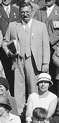
The French mathematician Louis Bachelier used a Wiener process in his 1900 thesis[287][288] in order to model price changes on the Paris Bourse, a stock exchange,[289] without knowing the work of Thiele.[21] It has been speculated that Bachelier drew ideas from the random walk model of Jules Regnault, but Bachelier did not cite him,[290] and Bachelier's thesis is now considered pioneering in the field of financial mathematics.[289][290]
It is commonly thought that Bachelier's work gained little attention and was forgotten for decades until it was rediscovered in the 1950s by the Leonard Savage, and then become more popular after Bachelier's thesis was translated into English in 1964. But the work was never forgotten in the mathematical community, as Bachelier published a book in 1912 detailing his ideas,[290] which was cited by mathematicians including Doob, Feller[290] and Kolmogorov.[21] The book continued to be cited, but then starting in the 1960s, the original thesis by Bachelier began to be cited more than his book when economists started citing Bachelier's work.[290]
In 1905, Albert Einstein published a paper where he studied the physical observation of Brownian motion or movement to explain the seemingly random movements of particles in liquids by using ideas from the kinetic theory of gases. Einstein derived a differential equation, known as a diffusion equation, for describing the probability of finding a particle in a certain region of space. Shortly after Einstein's first paper on Brownian movement, Marian Smoluchowski published work where he cited Einstein, but wrote that he had independently derived the equivalent results by using a different method.[291]
Einstein's work, as well as experimental results obtained by Jean Perrin, later inspired Norbert Wiener in the 1920s[292] to use a type of measure theory, developed by Percy Daniell, and Fourier analysis to prove the existence of the Wiener process as a mathematical object.[21]
Poisson process
[edit]The Poisson process is named after Siméon Poisson, due to its definition involving the Poisson distribution, but Poisson never studied the process.[22][293] There are a number of claims for early uses or discoveries of the Poisson process.[22][24] At the beginning of the 20th century, the Poisson process would arise independently in different situations.[22][24] In Sweden 1903, Filip Lundberg published a thesis containing work, now considered fundamental and pioneering, where he proposed to model insurance claims with a homogeneous Poisson process.[294][295]
Another discovery occurred in Denmark in 1909 when A.K. Erlang derived the Poisson distribution when developing a mathematical model for the number of incoming phone calls in a finite time interval. Erlang was not at the time aware of Poisson's earlier work and assumed that the number phone calls arriving in each interval of time were independent to each other. He then found the limiting case, which is effectively recasting the Poisson distribution as a limit of the binomial distribution.[22]
In 1910, Ernest Rutherford and Hans Geiger published experimental results on counting alpha particles. Motivated by their work, Harry Bateman studied the counting problem and derived Poisson probabilities as a solution to a family of differential equations, resulting in the independent discovery of the Poisson process.[22] After this time there were many studies and applications of the Poisson process, but its early history is complicated, which has been explained by the various applications of the process in numerous fields by biologists, ecologists, engineers and various physical scientists.[22]
Markov processes
[edit]Markov processes and Markov chains are named after Andrey Markov who studied Markov chains in the early 20th century. Markov was interested in studying an extension of independent random sequences. In his first paper on Markov chains, published in 1906, Markov showed that under certain conditions the average outcomes of the Markov chain would converge to a fixed vector of values, so proving a weak law of large numbers without the independence assumption,[296][297][298] which had been commonly regarded as a requirement for such mathematical laws to hold.[298] Markov later used Markov chains to study the distribution of vowels in Eugene Onegin, written by Alexander Pushkin, and proved a central limit theorem for such chains.
In 1912, Poincaré studied Markov chains on finite groups with an aim to study card shuffling. Other early uses of Markov chains include a diffusion model, introduced by Paul and Tatyana Ehrenfest in 1907, and a branching process, introduced by Francis Galton and Henry William Watson in 1873, preceding the work of Markov.[296][297] After the work of Galton and Watson, it was later revealed that their branching process had been independently discovered and studied around three decades earlier by Irénée-Jules Bienaymé.[299] Starting in 1928, Maurice Fréchet became interested in Markov chains, eventually resulting in him publishing in 1938 a detailed study on Markov chains.[296][300]
Andrei Kolmogorov developed in a 1931 paper a large part of the early theory of continuous-time Markov processes.[251][257] Kolmogorov was partly inspired by Louis Bachelier's 1900 work on fluctuations in the stock market as well as Norbert Wiener's work on Einstein's model of Brownian movement.[257][301] He introduced and studied a particular set of Markov processes known as diffusion processes, where he derived a set of differential equations describing the processes.[257][302] Independent of Kolmogorov's work, Sydney Chapman derived in a 1928 paper an equation, now called the Chapman–Kolmogorov equation, in a less mathematically rigorous way than Kolmogorov, while studying Brownian movement.[303] The differential equations are now called the Kolmogorov equations[304] or the Kolmogorov–Chapman equations.[305] Other mathematicians who contributed significantly to the foundations of Markov processes include William Feller, starting in the 1930s, and then later Eugene Dynkin, starting in the 1950s.[251]
Lévy processes
[edit]Lévy processes such as the Wiener process and the Poisson process (on the real line) are named after Paul Lévy who started studying them in the 1930s,[225] but they have connections to infinitely divisible distributions going back to the 1920s.[224] In a 1932 paper, Kolmogorov derived a characteristic function for random variables associated with Lévy processes. This result was later derived under more general conditions by Lévy in 1934, and then Khinchin independently gave an alternative form for this characteristic function in 1937.[251][306] In addition to Lévy, Khinchin and Kolomogrov, early fundamental contributions to the theory of Lévy processes were made by Bruno de Finetti and Kiyosi Itô.[224]
Mathematical construction
[edit]In mathematics, constructions of mathematical objects are needed, which is also the case for stochastic processes, to prove that they exist mathematically.[57] There are two main approaches for constructing a stochastic process. One approach involves considering a measurable space of functions, defining a suitable measurable mapping from a probability space to this measurable space of functions, and then deriving the corresponding finite-dimensional distributions.[307]
Another approach involves defining a collection of random variables to have specific finite-dimensional distributions, and then using Kolmogorov's existence theorem[j] to prove a corresponding stochastic process exists.[57][307] This theorem, which is an existence theorem for measures on infinite product spaces,[311] says that if any finite-dimensional distributions satisfy two conditions, known as consistency conditions, then there exists a stochastic process with those finite-dimensional distributions.[57]
Construction issues
[edit]When constructing continuous-time stochastic processes certain mathematical difficulties arise, due to the uncountable index sets, which do not occur with discrete-time processes.[58][59] One problem is that it is possible to have more than one stochastic process with the same finite-dimensional distributions. For example, both the left-continuous modification and the right-continuous modification of a Poisson process have the same finite-dimensional distributions.[312] This means that the distribution of the stochastic process does not, necessarily, specify uniquely the properties of the sample functions of the stochastic process.[307][313]
Another problem is that functionals of continuous-time process that rely upon an uncountable number of points of the index set may not be measurable, so the probabilities of certain events may not be well-defined.[168] For example, the supremum of a stochastic process or random field is not necessarily a well-defined random variable.[30][59] For a continuous-time stochastic process , other characteristics that depend on an uncountable number of points of the index set include:[168]
- a sample function of a stochastic process is a continuous function of ;
- a sample function of a stochastic process is a bounded function of ; and
- a sample function of a stochastic process is an increasing function of .
where the symbol ∈ can be read "a member of the set", as in a member of the set .
To overcome the two difficulties described above, i.e., "more than one..." and "functionals of...", different assumptions and approaches are possible.[69]
Resolving construction issues
[edit]One approach for avoiding mathematical construction issues of stochastic processes, proposed by Joseph Doob, is to assume that the stochastic process is separable.[314] Separability ensures that infinite-dimensional distributions determine the properties of sample functions by requiring that sample functions are essentially determined by their values on a dense countable set of points in the index set.[315] Furthermore, if a stochastic process is separable, then functionals of an uncountable number of points of the index set are measurable and their probabilities can be studied.[168][315]
Another approach is possible, originally developed by Anatoliy Skorokhod and Andrei Kolmogorov,[316] for a continuous-time stochastic process with any metric space as its state space. For the construction of such a stochastic process, it is assumed that the sample functions of the stochastic process belong to some suitable function space, which is usually the Skorokhod space consisting of all right-continuous functions with left limits. This approach is now more used than the separability assumption,[69][262] but such a stochastic process based on this approach will be automatically separable.[317]
Although less used, the separability assumption is considered more general because every stochastic process has a separable version.[262] It is also used when it is not possible to construct a stochastic process in a Skorokhod space.[173] For example, separability is assumed when constructing and studying random fields, where the collection of random variables is now indexed by sets other than the real line such as -dimensional Euclidean space.[30][318]
Application
[edit]Applications in Finance
[edit]Black-Scholes Model
[edit]One of the most famous applications of stochastic processes in finance is the Black-Scholes model for option pricing. Developed by Fischer Black, Myron Scholes, and Robert Solow, this model uses Geometric Brownian motion, a specific type of stochastic process, to describe the dynamics of asset prices.[319][320] The model assumes that the price of a stock follows a continuous-time stochastic process and provides a closed-form solution for pricing European-style options. The Black-Scholes formula has had a profound impact on financial markets, forming the basis for much of modern options trading.
The key assumption of the Black-Scholes model is that the price of a financial asset, such as a stock, follows a log-normal distribution, with its continuous returns following a normal distribution. Although the model has limitations, such as the assumption of constant volatility, it remains widely used due to its simplicity and practical relevance.
Stochastic Volatility Models
[edit]Another significant application of stochastic processes in finance is in stochastic volatility models, which aim to capture the time-varying nature of market volatility. The Heston model[321] is a popular example, allowing for the volatility of asset prices to follow its own stochastic process. Unlike the Black-Scholes model, which assumes constant volatility, stochastic volatility models provide a more flexible framework for modeling market dynamics, particularly during periods of high uncertainty or market stress.
Applications in Biology
[edit]Population Dynamics
[edit]One of the primary applications of stochastic processes in biology is in population dynamics. In contrast to deterministic models, which assume that populations change in predictable ways, stochastic models account for the inherent randomness in births, deaths, and migration. The birth-death process,[322] a simple stochastic model, describes how populations fluctuate over time due to random births and deaths. These models are particularly important when dealing with small populations, where random events can have large impacts, such as in the case of endangered species or small microbial populations.
Another example is the branching process,[322] which models the growth of a population where each individual reproduces independently. The branching process is often used to describe population extinction or explosion, particularly in epidemiology, where it can model the spread of infectious diseases within a population.
Applications in Computer Science
[edit]Randomized Algorithms
[edit]Stochastic processes play a critical role in computer science, particularly in the analysis and development of randomized algorithms. These algorithms utilize random inputs to simplify problem-solving or enhance performance in complex computational tasks. For instance, Markov chains are widely used in probabilistic algorithms for optimization and sampling tasks, such as those employed in search engines like Google's PageRank.[323] These methods balance computational efficiency with accuracy, making them invaluable for handling large datasets. Randomized algorithms are also extensively applied in areas such as cryptography, large-scale simulations, and artificial intelligence, where uncertainty must be managed effectively.[323]
Queuing Theory
[edit]Another significant application of stochastic processes in computer science is in queuing theory, which models the random arrival and service of tasks in a system.[324] This is particularly relevant in network traffic analysis and server management. For instance, queuing models help predict delays, manage resource allocation, and optimize throughput in web servers and communication networks. The flexibility of stochastic models allows researchers to simulate and improve the performance of high-traffic environments. For example, queueing theory is crucial for designing efficient data centers and cloud computing infrastructures.[325]
See also
[edit]- List of stochastic processes topics
- Covariance function
- Deterministic system
- Dynamics of Markovian particles
- Entropy rate (for a stochastic process)
- Ergodic process
- Gillespie algorithm
- Interacting particle system
- Markov chain
- Stochastic cellular automaton
- Random field
- Randomness
- Stationary process
- Statistical model
- Stochastic calculus
- Stochastic control
- Stochastic parrot
- Stochastic processes and boundary value problems
Notes
[edit]- ^ The term Brownian motion can refer to the physical process, also known as Brownian movement, and the stochastic process, a mathematical object, but to avoid ambiguity this article uses the terms Brownian motion process or Wiener process for the latter in a style similar to, for example, Gikhman and Skorokhod[19] or Rosenblatt.[20]
- ^ The term "separable" appears twice here with two different meanings, where the first meaning is from probability and the second from topology and analysis. For a stochastic process to be separable (in a probabilistic sense), its index set must be a separable space (in a topological or analytic sense), in addition to other conditions.[136]
- ^ The definition of separability for a continuous-time real-valued stochastic process can be stated in other ways.[172][173]
- ^ In the context of point processes, the term "state space" can mean the space on which the point process is defined such as the real line,[234][235] which corresponds to the index set in stochastic process terminology.
- ^ Also known as James or Jacques Bernoulli.[244]
- ^ It has been remarked that a notable exception was the St Petersburg School in Russia, where mathematicians led by Chebyshev studied probability theory.[249]
- ^ The name Khinchin is also written in (or transliterated into) English as Khintchine.[63]
- ^ Doob, when citing Khinchin, uses the term 'chance variable', which used to be an alternative term for 'random variable'.[260]
- ^ Later translated into English and published in 1950 as Foundations of the Theory of Probability[248]
- ^ The theorem has other names including Kolmogorov's consistency theorem,[308] Kolmogorov's extension theorem[309] or the Daniell–Kolmogorov theorem.[310]
References
[edit]- ^ a b c d e f g h i Joseph L. Doob (1990). Stochastic processes. Wiley. pp. 46, 47.
- ^ a b c d L. C. G. Rogers; David Williams (2000). Diffusions, Markov Processes, and Martingales: Volume 1, Foundations. Cambridge University Press. p. 1. ISBN 978-1-107-71749-7.
- ^ a b c J. Michael Steele (2012). Stochastic Calculus and Financial Applications. Springer Science & Business Media. p. 29. ISBN 978-1-4684-9305-4.
- ^ a b c d e Emanuel Parzen (2015). Stochastic Processes. Courier Dover Publications. pp. 7, 8. ISBN 978-0-486-79688-8.
- ^ a b c d e f g h i j k l Iosif Ilyich Gikhman; Anatoly Vladimirovich Skorokhod (1969). Introduction to the Theory of Random Processes. Courier Corporation. p. 1. ISBN 978-0-486-69387-3.
- ^ Bressloff, Paul C. (2014). Stochastic Processes in Cell Biology. Springer. ISBN 978-3-319-08488-6.
- ^ Van Kampen, N. G. (2011). Stochastic Processes in Physics and Chemistry. Elsevier. ISBN 978-0-08-047536-3.
- ^ Lande, Russell; Engen, Steinar; Sæther, Bernt-Erik (2003). Stochastic Population Dynamics in Ecology and Conservation. Oxford University Press. ISBN 978-0-19-852525-7.
- ^ Laing, Carlo; Lord, Gabriel J. (2010). Stochastic Methods in Neuroscience. Oxford University Press. ISBN 978-0-19-923507-0.
- ^ Paul, Wolfgang; Baschnagel, Jörg (2013). Stochastic Processes: From Physics to Finance. Springer Science+Business Media. ISBN 978-3-319-00327-6.
- ^ Dougherty, Edward R. (1999). Random processes for image and signal processing. SPIE Optical Engineering Press. ISBN 978-0-8194-2513-3.
- ^ Bertsekas, Dimitri P. (1996). Stochastic Optimal Control: The Discrete-Time Case. Athena Scientific. ISBN 1-886529-03-5.
- ^ Thomas M. Cover; Joy A. Thomas (2012). Elements of Information Theory. John Wiley & Sons. p. 71. ISBN 978-1-118-58577-1.
- ^ Baron, Michael (2015). Probability and Statistics for Computer Scientists (2nd ed.). CRC Press. p. 131. ISBN 978-1-4987-6060-7.
- ^ Baccelli, François; Blaszczyszyn, Bartlomiej (2009). Stochastic Geometry and Wireless Networks. Now Publishers Inc. ISBN 978-1-60198-264-3.
- ^ Steele, J. Michael (2001). Stochastic Calculus and Financial Applications. Springer Science+Business Media. ISBN 978-0-387-95016-7.
- ^ a b Musiela, Marek; Rutkowski, Marek (2006). Martingale Methods in Financial Modelling. Springer Science+Business Media. ISBN 978-3-540-26653-2.
- ^ Shreve, Steven E. (2004). Stochastic Calculus for Finance II: Continuous-Time Models. Springer Science+Business Media. ISBN 978-0-387-40101-0.
- ^ Iosif Ilyich Gikhman; Anatoly Vladimirovich Skorokhod (1969). Introduction to the Theory of Random Processes. Courier Corporation. ISBN 978-0-486-69387-3.
- ^ Murray Rosenblatt (1962). Random Processes. Oxford University Press.
- ^ a b c d e f g h i Jarrow, Robert; Protter, Philip (2004). "A short history of stochastic integration and mathematical finance: the early years, 1880–1970". A Festschrift for Herman Rubin. Institute of Mathematical Statistics Lecture Notes - Monograph Series. pp. 75–80. CiteSeerX 10.1.1.114.632. doi:10.1214/lnms/1196285381. ISBN 978-0-940600-61-4. ISSN 0749-2170.
- ^ a b c d e f g h Stirzaker, David (2000). "Advice to Hedgehogs, or, Constants Can Vary". The Mathematical Gazette. 84 (500): 197–210. doi:10.2307/3621649. ISSN 0025-5572. JSTOR 3621649. S2CID 125163415.
- ^ Donald L. Snyder; Michael I. Miller (2012). Random Point Processes in Time and Space. Springer Science & Business Media. p. 32. ISBN 978-1-4612-3166-0.
- ^ a b c d Guttorp, Peter; Thorarinsdottir, Thordis L. (2012). "What Happened to Discrete Chaos, the Quenouille Process, and the Sharp Markov Property? Some History of Stochastic Point Processes". International Statistical Review. 80 (2): 253–268. doi:10.1111/j.1751-5823.2012.00181.x. ISSN 0306-7734. S2CID 80836.
- ^ Gusak, Dmytro; Kukush, Alexander; Kulik, Alexey; Mishura, Yuliya; Pilipenko, Andrey (2010). Theory of Stochastic Processes: With Applications to Financial Mathematics and Risk Theory. Springer Science & Business Media. p. 21. ISBN 978-0-387-87862-1.
- ^ Valeriy Skorokhod (2005). Basic Principles and Applications of Probability Theory. Springer Science & Business Media. p. 42. ISBN 978-3-540-26312-8.
- ^ a b c d e f Olav Kallenberg (2002). Foundations of Modern Probability. Springer Science & Business Media. pp. 24–25. ISBN 978-0-387-95313-7.
- ^ a b c d e f g h i j k l m n o p John Lamperti (1977). Stochastic processes: a survey of the mathematical theory. Springer-Verlag. pp. 1–2. ISBN 978-3-540-90275-1.
- ^ a b c d Loïc Chaumont; Marc Yor (2012). Exercises in Probability: A Guided Tour from Measure Theory to Random Processes, Via Conditioning. Cambridge University Press. p. 175. ISBN 978-1-107-60655-5.
- ^ a b c d e f g h Robert J. Adler; Jonathan E. Taylor (2009). Random Fields and Geometry. Springer Science & Business Media. pp. 7–8. ISBN 978-0-387-48116-6.
- ^ Gregory F. Lawler; Vlada Limic (2010). Random Walk: A Modern Introduction. Cambridge University Press. ISBN 978-1-139-48876-1.
- ^ David Williams (1991). Probability with Martingales. Cambridge University Press. ISBN 978-0-521-40605-5.
- ^ L. C. G. Rogers; David Williams (2000). Diffusions, Markov Processes, and Martingales: Volume 1, Foundations. Cambridge University Press. ISBN 978-1-107-71749-7.
- ^ David Applebaum (2004). Lévy Processes and Stochastic Calculus. Cambridge University Press. ISBN 978-0-521-83263-2.
- ^ Mikhail Lifshits (2012). Lectures on Gaussian Processes. Springer Science & Business Media. ISBN 978-3-642-24939-6.
- ^ Robert J. Adler (2010). The Geometry of Random Fields. SIAM. ISBN 978-0-89871-693-1.
- ^ Samuel Karlin; Howard E. Taylor (2012). A First Course in Stochastic Processes. Academic Press. ISBN 978-0-08-057041-9.
- ^ Bruce Hajek (2015). Random Processes for Engineers. Cambridge University Press. ISBN 978-1-316-24124-0.
- ^ a b G. Latouche; V. Ramaswami (1999). Introduction to Matrix Analytic Methods in Stochastic Modeling. SIAM. ISBN 978-0-89871-425-8.
- ^ D.J. Daley; David Vere-Jones (2007). An Introduction to the Theory of Point Processes: Volume II: General Theory and Structure. Springer Science & Business Media. ISBN 978-0-387-21337-8.
- ^ Patrick Billingsley (2008). Probability and Measure. Wiley India Pvt. Limited. ISBN 978-81-265-1771-8.
- ^ Pierre Brémaud (2014). Fourier Analysis and Stochastic Processes. Springer. ISBN 978-3-319-09590-5.
- ^ Adam Bobrowski (2005). Functional Analysis for Probability and Stochastic Processes: An Introduction. Cambridge University Press. ISBN 978-0-521-83166-6.
- ^ Applebaum, David (2004). "Lévy processes: From probability to finance and quantum groups". Notices of the AMS. 51 (11): 1336–1347.
- ^ a b Jochen Blath; Peter Imkeller; Sylvie Roelly (2011). Surveys in Stochastic Processes. European Mathematical Society. ISBN 978-3-03719-072-2.
- ^ Michel Talagrand (2014). Upper and Lower Bounds for Stochastic Processes: Modern Methods and Classical Problems. Springer Science & Business Media. pp. 4–. ISBN 978-3-642-54075-2.
- ^ Paul C. Bressloff (2014). Stochastic Processes in Cell Biology. Springer. pp. vii–ix. ISBN 978-3-319-08488-6.
- ^ a b c d Samuel Karlin; Howard E. Taylor (2012). A First Course in Stochastic Processes. Academic Press. p. 27. ISBN 978-0-08-057041-9.
- ^ a b c d e f g h i j Applebaum, David (2004). "Lévy processes: From probability to finance and quantum groups". Notices of the AMS. 51 (11): 1337.
- ^ a b L. C. G. Rogers; David Williams (2000). Diffusions, Markov Processes, and Martingales: Volume 1, Foundations. Cambridge University Press. pp. 121–124. ISBN 978-1-107-71749-7.
- ^ a b c d e f Ionut Florescu (2014). Probability and Stochastic Processes. John Wiley & Sons. pp. 294, 295. ISBN 978-1-118-59320-2.
- ^ a b Samuel Karlin; Howard E. Taylor (2012). A First Course in Stochastic Processes. Academic Press. p. 26. ISBN 978-0-08-057041-9.
- ^ Donald L. Snyder; Michael I. Miller (2012). Random Point Processes in Time and Space. Springer Science & Business Media. pp. 24, 25. ISBN 978-1-4612-3166-0.
- ^ a b Patrick Billingsley (2008). Probability and Measure. Wiley India Pvt. Limited. p. 482. ISBN 978-81-265-1771-8.
- ^ a b Alexander A. Borovkov (2013). Probability Theory. Springer Science & Business Media. p. 527. ISBN 978-1-4471-5201-9.
- ^ a b c Pierre Brémaud (2014). Fourier Analysis and Stochastic Processes. Springer. p. 120. ISBN 978-3-319-09590-5.
- ^ a b c d e Jeffrey S Rosenthal (2006). A First Look at Rigorous Probability Theory. World Scientific Publishing Co Inc. pp. 177–178. ISBN 978-981-310-165-4.
- ^ a b Peter E. Kloeden; Eckhard Platen (2013). Numerical Solution of Stochastic Differential Equations. Springer Science & Business Media. p. 63. ISBN 978-3-662-12616-5.
- ^ a b c Davar Khoshnevisan (2006). Multiparameter Processes: An Introduction to Random Fields. Springer Science & Business Media. pp. 153–155. ISBN 978-0-387-21631-7.
- ^ a b "Stochastic". Oxford English Dictionary (Online ed.). Oxford University Press. (Subscription or participating institution membership required.)
- ^ O. B. Sheĭnin (2006). Theory of probability and statistics as exemplified in short dictums. NG Verlag. p. 5. ISBN 978-3-938417-40-9.
- ^ Oscar Sheynin; Heinrich Strecker (2011). Alexandr A. Chuprov: Life, Work, Correspondence. V&R unipress GmbH. p. 136. ISBN 978-3-89971-812-6.
- ^ a b c d Doob, Joseph (1934). "Stochastic Processes and Statistics". Proceedings of the National Academy of Sciences of the United States of America. 20 (6): 376–379. Bibcode:1934PNAS...20..376D. doi:10.1073/pnas.20.6.376. PMC 1076423. PMID 16587907.
- ^ Khintchine, A. (1934). "Korrelationstheorie der stationeren stochastischen Prozesse". Mathematische Annalen. 109 (1): 604–615. doi:10.1007/BF01449156. ISSN 0025-5831. S2CID 122842868.
- ^ Kolmogoroff, A. (1931). "Über die analytischen Methoden in der Wahrscheinlichkeitsrechnung". Mathematische Annalen. 104 (1): 1. doi:10.1007/BF01457949. ISSN 0025-5831. S2CID 119439925.
- ^ "Random". Oxford English Dictionary (Online ed.). Oxford University Press. (Subscription or participating institution membership required.)
- ^ Bert E. Fristedt; Lawrence F. Gray (2013). A Modern Approach to Probability Theory. Springer Science & Business Media. p. 580. ISBN 978-1-4899-2837-5.
- ^ a b c d L. C. G. Rogers; David Williams (2000). Diffusions, Markov Processes, and Martingales: Volume 1, Foundations. Cambridge University Press. pp. 121, 122. ISBN 978-1-107-71749-7.
- ^ a b c d e Søren Asmussen (2003). Applied Probability and Queues. Springer Science & Business Media. p. 408. ISBN 978-0-387-00211-8.
- ^ a b David Stirzaker (2005). Stochastic Processes and Models. Oxford University Press. p. 45. ISBN 978-0-19-856814-8.
- ^ Murray Rosenblatt (1962). Random Processes. Oxford University Press. p. 91.
- ^ John A. Gubner (2006). Probability and Random Processes for Electrical and Computer Engineers. Cambridge University Press. p. 383. ISBN 978-1-139-45717-0.
- ^ a b Kiyosi Itō (2006). Essentials of Stochastic Processes. American Mathematical Soc. p. 13. ISBN 978-0-8218-3898-3.
- ^ M. Loève (1978). Probability Theory II. Springer Science & Business Media. p. 163. ISBN 978-0-387-90262-3.
- ^ Pierre Brémaud (2014). Fourier Analysis and Stochastic Processes. Springer. p. 133. ISBN 978-3-319-09590-5.
- ^ a b Gusak et al. (2010), p. 1
- ^ Richard F. Bass (2011). Stochastic Processes. Cambridge University Press. p. 1. ISBN 978-1-139-50147-7.
- ^ a b ,John Lamperti (1977). Stochastic processes: a survey of the mathematical theory. Springer-Verlag. p. 3. ISBN 978-3-540-90275-1.
- ^ Fima C. Klebaner (2005). Introduction to Stochastic Calculus with Applications. Imperial College Press. p. 55. ISBN 978-1-86094-555-7.
- ^ a b Ionut Florescu (2014). Probability and Stochastic Processes. John Wiley & Sons. p. 293. ISBN 978-1-118-59320-2.
- ^ a b Florescu, Ionut (2014). Probability and Stochastic Processes. John Wiley & Sons. p. 301. ISBN 978-1-118-59320-2.
- ^ a b Bertsekas, Dimitri P.; Tsitsiklis, John N. (2002). Introduction to Probability. Athena Scientific. p. 273. ISBN 978-1-886529-40-3.
- ^ Ibe, Oliver C. (2013). Elements of Random Walk and Diffusion Processes. John Wiley & Sons. p. 11. ISBN 978-1-118-61793-9.
- ^ Achim Klenke (2013). Probability Theory: A Comprehensive Course. Springer. p. 347. ISBN 978-1-4471-5362-7.
- ^ Gregory F. Lawler; Vlada Limic (2010). Random Walk: A Modern Introduction. Cambridge University Press. p. 1. ISBN 978-1-139-48876-1.
- ^ Olav Kallenberg (2002). Foundations of Modern Probability. Springer Science & Business Media. p. 136. ISBN 978-0-387-95313-7.
- ^ Ionut Florescu (2014). Probability and Stochastic Processes. John Wiley & Sons. p. 383. ISBN 978-1-118-59320-2.
- ^ Rick Durrett (2010). Probability: Theory and Examples. Cambridge University Press. p. 277. ISBN 978-1-139-49113-6.
- ^ a b c Weiss, George H. (2006). "Random Walks". Encyclopedia of Statistical Sciences. p. 1. doi:10.1002/0471667196.ess2180.pub2. ISBN 978-0471667193.
- ^ Aris Spanos (1999). Probability Theory and Statistical Inference: Econometric Modeling with Observational Data. Cambridge University Press. p. 454. ISBN 978-0-521-42408-0.
- ^ a b Fima C. Klebaner (2005). Introduction to Stochastic Calculus with Applications. Imperial College Press. p. 81. ISBN 978-1-86094-555-7.
- ^ Allan Gut (2012). Probability: A Graduate Course. Springer Science & Business Media. p. 88. ISBN 978-1-4614-4708-5.
- ^ Geoffrey Grimmett; David Stirzaker (2001). Probability and Random Processes. OUP Oxford. p. 71. ISBN 978-0-19-857222-0.
- ^ Fima C. Klebaner (2005). Introduction to Stochastic Calculus with Applications. Imperial College Press. p. 56. ISBN 978-1-86094-555-7.
- ^ Brush, Stephen G. (1968). "A history of random processes". Archive for History of Exact Sciences. 5 (1): 1–2. doi:10.1007/BF00328110. ISSN 0003-9519. S2CID 117623580.
- ^ Applebaum, David (2004). "Lévy processes: From probability to finance and quantum groups". Notices of the AMS. 51 (11): 1338.
- ^ Iosif Ilyich Gikhman; Anatoly Vladimirovich Skorokhod (1969). Introduction to the Theory of Random Processes. Courier Corporation. p. 21. ISBN 978-0-486-69387-3.
- ^ Ionut Florescu (2014). Probability and Stochastic Processes. John Wiley & Sons. p. 471. ISBN 978-1-118-59320-2.
- ^ a b Samuel Karlin; Howard E. Taylor (2012). A First Course in Stochastic Processes. Academic Press. pp. 21, 22. ISBN 978-0-08-057041-9.
- ^ Ioannis Karatzas; Steven Shreve (1991). Brownian Motion and Stochastic Calculus. Springer. p. VIII. ISBN 978-1-4612-0949-2.
- ^ Daniel Revuz; Marc Yor (2013). Continuous Martingales and Brownian Motion. Springer Science & Business Media. p. IX. ISBN 978-3-662-06400-9.
- ^ Jeffrey S Rosenthal (2006). A First Look at Rigorous Probability Theory. World Scientific Publishing Co Inc. p. 186. ISBN 978-981-310-165-4.
- ^ Donald L. Snyder; Michael I. Miller (2012). Random Point Processes in Time and Space. Springer Science & Business Media. p. 33. ISBN 978-1-4612-3166-0.
- ^ J. Michael Steele (2012). Stochastic Calculus and Financial Applications. Springer Science & Business Media. p. 118. ISBN 978-1-4684-9305-4.
- ^ a b Peter Mörters; Yuval Peres (2010). Brownian Motion. Cambridge University Press. pp. 1, 3. ISBN 978-1-139-48657-6.
- ^ Ioannis Karatzas; Steven Shreve (1991). Brownian Motion and Stochastic Calculus. Springer. p. 78. ISBN 978-1-4612-0949-2.
- ^ Ioannis Karatzas; Steven Shreve (1991). Brownian Motion and Stochastic Calculus. Springer. p. 61. ISBN 978-1-4612-0949-2.
- ^ Steven E. Shreve (2004). Stochastic Calculus for Finance II: Continuous-Time Models. Springer Science & Business Media. p. 93. ISBN 978-0-387-40101-0.
- ^ Olav Kallenberg (2002). Foundations of Modern Probability. Springer Science & Business Media. pp. 225, 260. ISBN 978-0-387-95313-7.
- ^ Ioannis Karatzas; Steven Shreve (1991). Brownian Motion and Stochastic Calculus. Springer. p. 70. ISBN 978-1-4612-0949-2.
- ^ Peter Mörters; Yuval Peres (2010). Brownian Motion. Cambridge University Press. p. 131. ISBN 978-1-139-48657-6.
- ^ Fima C. Klebaner (2005). Introduction to Stochastic Calculus with Applications. Imperial College Press. ISBN 978-1-86094-555-7.
- ^ Ioannis Karatzas; Steven Shreve (1991). Brownian Motion and Stochastic Calculus. Springer. ISBN 978-1-4612-0949-2.
- ^ Applebaum, David (2004). "Lévy processes: From probability to finance and quantum groups". Notices of the AMS. 51 (11): 1341.
- ^ Samuel Karlin; Howard E. Taylor (2012). A First Course in Stochastic Processes. Academic Press. p. 340. ISBN 978-0-08-057041-9.
- ^ Fima C. Klebaner (2005). Introduction to Stochastic Calculus with Applications. Imperial College Press. p. 124. ISBN 978-1-86094-555-7.
- ^ Ioannis Karatzas; Steven Shreve (1991). Brownian Motion and Stochastic Calculus. Springer. p. 47. ISBN 978-1-4612-0949-2.
- ^ Ubbo F. Wiersema (2008). Brownian Motion Calculus. John Wiley & Sons. p. 2. ISBN 978-0-470-02171-2.
- ^ a b c Henk C. Tijms (2003). A First Course in Stochastic Models. Wiley. pp. 1, 2. ISBN 978-0-471-49881-0.
- ^ D.J. Daley; D. Vere-Jones (2006). An Introduction to the Theory of Point Processes: Volume I: Elementary Theory and Methods. Springer Science & Business Media. pp. 19–36. ISBN 978-0-387-21564-8.
- ^ Mark A. Pinsky; Samuel Karlin (2011). An Introduction to Stochastic Modeling. Academic Press. p. 241. ISBN 978-0-12-381416-6.
- ^ J. F. C. Kingman (1992). Poisson Processes. Clarendon Press. p. 38. ISBN 978-0-19-159124-2.
- ^ D.J. Daley; D. Vere-Jones (2006). An Introduction to the Theory of Point Processes: Volume I: Elementary Theory and Methods. Springer Science & Business Media. p. 19. ISBN 978-0-387-21564-8.
- ^ J. F. C. Kingman (1992). Poisson Processes. Clarendon Press. p. 22. ISBN 978-0-19-159124-2.
- ^ Samuel Karlin; Howard E. Taylor (2012). A First Course in Stochastic Processes. Academic Press. pp. 118, 119. ISBN 978-0-08-057041-9.
- ^ Leonard Kleinrock (1976). Queueing Systems: Theory. Wiley. p. 61. ISBN 978-0-471-49110-1.
- ^ Murray Rosenblatt (1962). Random Processes. Oxford University Press. p. 94.
- ^ a b Martin Haenggi (2013). Stochastic Geometry for Wireless Networks. Cambridge University Press. pp. 10, 18. ISBN 978-1-107-01469-5.
- ^ a b Sung Nok Chiu; Dietrich Stoyan; Wilfrid S. Kendall; Joseph Mecke (2013). Stochastic Geometry and Its Applications. John Wiley & Sons. pp. 41, 108. ISBN 978-1-118-65825-3.
- ^ J. F. C. Kingman (1992). Poisson Processes. Clarendon Press. p. 11. ISBN 978-0-19-159124-2.
- ^ a b Roy L. Streit (2010). Poisson Point Processes: Imaging, Tracking, and Sensing. Springer Science & Business Media. p. 1. ISBN 978-1-4419-6923-1.
- ^ J. F. C. Kingman (1992). Poisson Processes. Clarendon Press. p. v. ISBN 978-0-19-159124-2.
- ^ a b Alexander A. Borovkov (2013). Probability Theory. Springer Science & Business Media. p. 528. ISBN 978-1-4471-5201-9.
- ^ Georg Lindgren; Holger Rootzen; Maria Sandsten (2013). Stationary Stochastic Processes for Scientists and Engineers. CRC Press. p. 11. ISBN 978-1-4665-8618-5.
- ^ Aumann, Robert (December 1961). "Borel structures for function spaces". Illinois Journal of Mathematics. 5 (4). doi:10.1215/ijm/1255631584. S2CID 117171116.
- ^ a b c Valeriy Skorokhod (2005). Basic Principles and Applications of Probability Theory. Springer Science & Business Media. pp. 93, 94. ISBN 978-3-540-26312-8.
- ^ Donald L. Snyder; Michael I. Miller (2012). Random Point Processes in Time and Space. Springer Science & Business Media. p. 25. ISBN 978-1-4612-3166-0.
- ^ Valeriy Skorokhod (2005). Basic Principles and Applications of Probability Theory. Springer Science & Business Media. p. 104. ISBN 978-3-540-26312-8.
- ^ Ionut Florescu (2014). Probability and Stochastic Processes. John Wiley & Sons. p. 296. ISBN 978-1-118-59320-2.
- ^ Patrick Billingsley (2008). Probability and Measure. Wiley India Pvt. Limited. p. 493. ISBN 978-81-265-1771-8.
- ^ Bernt Øksendal (2003). Stochastic Differential Equations: An Introduction with Applications. Springer Science & Business Media. p. 10. ISBN 978-3-540-04758-2.
- ^ a b c d e Peter K. Friz; Nicolas B. Victoir (2010). Multidimensional Stochastic Processes as Rough Paths: Theory and Applications. Cambridge University Press. p. 571. ISBN 978-1-139-48721-4.
- ^ Sidney I. Resnick (2013). Adventures in Stochastic Processes. Springer Science & Business Media. pp. 40–41. ISBN 978-1-4612-0387-2.
- ^ Ward Whitt (2006). Stochastic-Process Limits: An Introduction to Stochastic-Process Limits and Their Application to Queues. Springer Science & Business Media. p. 23. ISBN 978-0-387-21748-2.
- ^ David Applebaum (2004). Lévy Processes and Stochastic Calculus. Cambridge University Press. p. 4. ISBN 978-0-521-83263-2.
- ^ Daniel Revuz; Marc Yor (2013). Continuous Martingales and Brownian Motion. Springer Science & Business Media. p. 10. ISBN 978-3-662-06400-9.
- ^ L. C. G. Rogers; David Williams (2000). Diffusions, Markov Processes, and Martingales: Volume 1, Foundations. Cambridge University Press. p. 123. ISBN 978-1-107-71749-7.
- ^ a b c d John Lamperti (1977). Stochastic processes: a survey of the mathematical theory. Springer-Verlag. pp. 6 and 7. ISBN 978-3-540-90275-1.
- ^ Iosif I. Gikhman; Anatoly Vladimirovich Skorokhod (1969). Introduction to the Theory of Random Processes. Courier Corporation. p. 4. ISBN 978-0-486-69387-3.
- ^ a b c d Robert J. Adler (2010). The Geometry of Random Fields. SIAM. pp. 14, 15. ISBN 978-0-89871-693-1.
- ^ Sung Nok Chiu; Dietrich Stoyan; Wilfrid S. Kendall; Joseph Mecke (2013). Stochastic Geometry and Its Applications. John Wiley & Sons. p. 112. ISBN 978-1-118-65825-3.
- ^ a b Joseph L. Doob (1990). Stochastic processes. Wiley. pp. 94–96.
- ^ a b Ionut Florescu (2014). Probability and Stochastic Processes. John Wiley & Sons. pp. 298, 299. ISBN 978-1-118-59320-2.
- ^ Iosif Ilyich Gikhman; Anatoly Vladimirovich Skorokhod (1969). Introduction to the Theory of Random Processes. Courier Corporation. p. 8. ISBN 978-0-486-69387-3.
- ^ a b c David Williams (1991). Probability with Martingales. Cambridge University Press. pp. 93, 94. ISBN 978-0-521-40605-5.
- ^ Fima C. Klebaner (2005). Introduction to Stochastic Calculus with Applications. Imperial College Press. pp. 22–23. ISBN 978-1-86094-555-7.
- ^ Peter Mörters; Yuval Peres (2010). Brownian Motion. Cambridge University Press. p. 37. ISBN 978-1-139-48657-6.
- ^ a b L. C. G. Rogers; David Williams (2000). Diffusions, Markov Processes, and Martingales: Volume 1, Foundations. Cambridge University Press. p. 130. ISBN 978-1-107-71749-7.
- ^ Alexander A. Borovkov (2013). Probability Theory. Springer Science & Business Media. p. 530. ISBN 978-1-4471-5201-9.
- ^ Fima C. Klebaner (2005). Introduction to Stochastic Calculus with Applications. Imperial College Press. p. 48. ISBN 978-1-86094-555-7.
- ^ a b Bernt Øksendal (2003). Stochastic Differential Equations: An Introduction with Applications. Springer Science & Business Media. p. 14. ISBN 978-3-540-04758-2.
- ^ a b Ionut Florescu (2014). Probability and Stochastic Processes. John Wiley & Sons. p. 472. ISBN 978-1-118-59320-2.
- ^ Daniel Revuz; Marc Yor (2013). Continuous Martingales and Brownian Motion. Springer Science & Business Media. pp. 18–19. ISBN 978-3-662-06400-9.
- ^ David Applebaum (2004). Lévy Processes and Stochastic Calculus. Cambridge University Press. p. 20. ISBN 978-0-521-83263-2.
- ^ Hiroshi Kunita (1997). Stochastic Flows and Stochastic Differential Equations. Cambridge University Press. p. 31. ISBN 978-0-521-59925-2.
- ^ Olav Kallenberg (2002). Foundations of Modern Probability. Springer Science & Business Media. p. 35. ISBN 978-0-387-95313-7.
- ^ Monique Jeanblanc; Marc Yor; Marc Chesney (2009). Mathematical Methods for Financial Markets. Springer Science & Business Media. p. 11. ISBN 978-1-85233-376-8.
- ^ a b c d e f Kiyosi Itō (2006). Essentials of Stochastic Processes. American Mathematical Soc. pp. 32–33. ISBN 978-0-8218-3898-3.
- ^ Iosif Ilyich Gikhman; Anatoly Vladimirovich Skorokhod (1969). Introduction to the Theory of Random Processes. Courier Corporation. p. 150. ISBN 978-0-486-69387-3.
- ^ a b Petar Todorovic (2012). An Introduction to Stochastic Processes and Their Applications. Springer Science & Business Media. pp. 19–20. ISBN 978-1-4613-9742-7.
- ^ Ilya Molchanov (2005). Theory of Random Sets. Springer Science & Business Media. p. 340. ISBN 978-1-85233-892-3.
- ^ a b Patrick Billingsley (2008). Probability and Measure. Wiley India Pvt. Limited. pp. 526–527. ISBN 978-81-265-1771-8.
- ^ a b Alexander A. Borovkov (2013). Probability Theory. Springer Science & Business Media. p. 535. ISBN 978-1-4471-5201-9.
- ^ Gusak et al. (2010), p. 22
- ^ Joseph L. Doob (1990). Stochastic processes. Wiley. p. 56.
- ^ Davar Khoshnevisan (2006). Multiparameter Processes: An Introduction to Random Fields. Springer Science & Business Media. p. 155. ISBN 978-0-387-21631-7.
- ^ Lapidoth, Amos, A Foundation in Digital Communication, Cambridge University Press, 2009.
- ^ a b c Kun Il Park, Fundamentals of Probability and Stochastic Processes with Applications to Communications, Springer, 2018, 978-3-319-68074-3
- ^ a b c d Ward Whitt (2006). Stochastic-Process Limits: An Introduction to Stochastic-Process Limits and Their Application to Queues. Springer Science & Business Media. pp. 78–79. ISBN 978-0-387-21748-2.
- ^ a b Gusak et al. (2010), p. 24
- ^ a b c d Vladimir I. Bogachev (2007). Measure Theory (Volume 2). Springer Science & Business Media. p. 53. ISBN 978-3-540-34514-5.
- ^ a b c Fima C. Klebaner (2005). Introduction to Stochastic Calculus with Applications. Imperial College Press. p. 4. ISBN 978-1-86094-555-7.
- ^ a b Søren Asmussen (2003). Applied Probability and Queues. Springer Science & Business Media. p. 420. ISBN 978-0-387-00211-8.
- ^ a b c Patrick Billingsley (2013). Convergence of Probability Measures. John Wiley & Sons. p. 121. ISBN 978-1-118-62596-5.
- ^ Richard F. Bass (2011). Stochastic Processes. Cambridge University Press. p. 34. ISBN 978-1-139-50147-7.
- ^ Nicholas H. Bingham; Rüdiger Kiesel (2013). Risk-Neutral Valuation: Pricing and Hedging of Financial Derivatives. Springer Science & Business Media. p. 154. ISBN 978-1-4471-3856-3.
- ^ Alexander A. Borovkov (2013). Probability Theory. Springer Science & Business Media. p. 532. ISBN 978-1-4471-5201-9.
- ^ Davar Khoshnevisan (2006). Multiparameter Processes: An Introduction to Random Fields. Springer Science & Business Media. pp. 148–165. ISBN 978-0-387-21631-7.
- ^ Petar Todorovic (2012). An Introduction to Stochastic Processes and Their Applications. Springer Science & Business Media. p. 22. ISBN 978-1-4613-9742-7.
- ^ Ward Whitt (2006). Stochastic-Process Limits: An Introduction to Stochastic-Process Limits and Their Application to Queues. Springer Science & Business Media. p. 79. ISBN 978-0-387-21748-2.
- ^ Richard Serfozo (2009). Basics of Applied Stochastic Processes. Springer Science & Business Media. p. 2. ISBN 978-3-540-89332-5.
- ^ Y.A. Rozanov (2012). Markov Random Fields. Springer Science & Business Media. p. 58. ISBN 978-1-4613-8190-7.
- ^ Sheldon M. Ross (1996). Stochastic processes. Wiley. pp. 235, 358. ISBN 978-0-471-12062-9.
- ^ Ionut Florescu (2014). Probability and Stochastic Processes. John Wiley & Sons. pp. 373, 374. ISBN 978-1-118-59320-2.
- ^ a b Samuel Karlin; Howard E. Taylor (2012). A First Course in Stochastic Processes. Academic Press. p. 49. ISBN 978-0-08-057041-9.
- ^ a b Søren Asmussen (2003). Applied Probability and Queues. Springer Science & Business Media. p. 7. ISBN 978-0-387-00211-8.
- ^ Emanuel Parzen (2015). Stochastic Processes. Courier Dover Publications. p. 188. ISBN 978-0-486-79688-8.
- ^ Samuel Karlin; Howard E. Taylor (2012). A First Course in Stochastic Processes. Academic Press. pp. 29, 30. ISBN 978-0-08-057041-9.
- ^ John Lamperti (1977). Stochastic processes: a survey of the mathematical theory. Springer-Verlag. pp. 106–121. ISBN 978-3-540-90275-1.
- ^ Sheldon M. Ross (1996). Stochastic processes. Wiley. pp. 174, 231. ISBN 978-0-471-12062-9.
- ^ Sean Meyn; Richard L. Tweedie (2009). Markov Chains and Stochastic Stability. Cambridge University Press. p. 19. ISBN 978-0-521-73182-9.
- ^ Samuel Karlin; Howard E. Taylor (2012). A First Course in Stochastic Processes. Academic Press. p. 47. ISBN 978-0-08-057041-9.
- ^ Reuven Y. Rubinstein; Dirk P. Kroese (2011). Simulation and the Monte Carlo Method. John Wiley & Sons. p. 225. ISBN 978-1-118-21052-9.
- ^ Dani Gamerman; Hedibert F. Lopes (2006). Markov Chain Monte Carlo: Stochastic Simulation for Bayesian Inference, Second Edition. CRC Press. ISBN 978-1-58488-587-0.
- ^ Y.A. Rozanov (2012). Markov Random Fields. Springer Science & Business Media. p. 61. ISBN 978-1-4613-8190-7.
- ^ Donald L. Snyder; Michael I. Miller (2012). Random Point Processes in Time and Space. Springer Science & Business Media. p. 27. ISBN 978-1-4612-3166-0.
- ^ Pierre Bremaud (2013). Markov Chains: Gibbs Fields, Monte Carlo Simulation, and Queues. Springer Science & Business Media. p. 253. ISBN 978-1-4757-3124-8.
- ^ a b c Fima C. Klebaner (2005). Introduction to Stochastic Calculus with Applications. Imperial College Press. p. 65. ISBN 978-1-86094-555-7.
- ^ a b c Ioannis Karatzas; Steven Shreve (1991). Brownian Motion and Stochastic Calculus. Springer. p. 11. ISBN 978-1-4612-0949-2.
- ^ Joseph L. Doob (1990). Stochastic processes. Wiley. pp. 292, 293.
- ^ Gilles Pisier (2016). Martingales in Banach Spaces. Cambridge University Press. ISBN 978-1-316-67946-3.
- ^ a b J. Michael Steele (2012). Stochastic Calculus and Financial Applications. Springer Science & Business Media. pp. 12, 13. ISBN 978-1-4684-9305-4.
- ^ a b P. Hall; C. C. Heyde (2014). Martingale Limit Theory and Its Application. Elsevier Science. p. 2. ISBN 978-1-4832-6322-9.
- ^ J. Michael Steele (2012). Stochastic Calculus and Financial Applications. Springer Science & Business Media. p. 115. ISBN 978-1-4684-9305-4.
- ^ Sheldon M. Ross (1996). Stochastic processes. Wiley. p. 295. ISBN 978-0-471-12062-9.
- ^ a b J. Michael Steele (2012). Stochastic Calculus and Financial Applications. Springer Science & Business Media. p. 11. ISBN 978-1-4684-9305-4.
- ^ Olav Kallenberg (2002). Foundations of Modern Probability. Springer Science & Business Media. p. 96. ISBN 978-0-387-95313-7.
- ^ J. Michael Steele (2012). Stochastic Calculus and Financial Applications. Springer Science & Business Media. p. 371. ISBN 978-1-4684-9305-4.
- ^ J. Michael Steele (2012). Stochastic Calculus and Financial Applications. Springer Science & Business Media. p. 22. ISBN 978-1-4684-9305-4.
- ^ Geoffrey Grimmett; David Stirzaker (2001). Probability and Random Processes. OUP Oxford. p. 336. ISBN 978-0-19-857222-0.
- ^ Glasserman, Paul; Kou, Steven (2006). "A Conversation with Chris Heyde". Statistical Science. 21 (2): 292, 293. arXiv:math/0609294. Bibcode:2006math......9294G. doi:10.1214/088342306000000088. ISSN 0883-4237. S2CID 62552177.
- ^ Francois Baccelli; Pierre Bremaud (2013). Elements of Queueing Theory: Palm Martingale Calculus and Stochastic Recurrences. Springer Science & Business Media. ISBN 978-3-662-11657-9.
- ^ P. Hall; C. C. Heyde (2014). Martingale Limit Theory and Its Application. Elsevier Science. p. x. ISBN 978-1-4832-6322-9.
- ^ a b c d Jean Bertoin (1998). Lévy Processes. Cambridge University Press. p. viii. ISBN 978-0-521-64632-1.
- ^ a b c Applebaum, David (2004). "Lévy processes: From probability to finance and quantum groups". Notices of the AMS. 51 (11): 1336.
- ^ David Applebaum (2004). Lévy Processes and Stochastic Calculus. Cambridge University Press. p. 69. ISBN 978-0-521-83263-2.
- ^ Leonid Koralov; Yakov G. Sinai (2007). Theory of Probability and Random Processes. Springer Science & Business Media. p. 171. ISBN 978-3-540-68829-7.
- ^ David Applebaum (2004). Lévy Processes and Stochastic Calculus. Cambridge University Press. p. 19. ISBN 978-0-521-83263-2.
- ^ Sung Nok Chiu; Dietrich Stoyan; Wilfrid S. Kendall; Joseph Mecke (2013). Stochastic Geometry and Its Applications. John Wiley & Sons. p. 109. ISBN 978-1-118-65825-3.
- ^ Sung Nok Chiu; Dietrich Stoyan; Wilfrid S. Kendall; Joseph Mecke (2013). Stochastic Geometry and Its Applications. John Wiley & Sons. p. 108. ISBN 978-1-118-65825-3.
- ^ Martin Haenggi (2013). Stochastic Geometry for Wireless Networks. Cambridge University Press. p. 10. ISBN 978-1-107-01469-5.
- ^ D.J. Daley; D. Vere-Jones (2006). An Introduction to the Theory of Point Processes: Volume I: Elementary Theory and Methods. Springer Science & Business Media. p. 194. ISBN 978-0-387-21564-8.
- ^ a b c Cox, D. R.; Isham, Valerie (1980). Point Processes. CRC Press. p. 3. ISBN 978-0-412-21910-8.
- ^ J. F. C. Kingman (1992). Poisson Processes. Clarendon Press. p. 8. ISBN 978-0-19-159124-2.
- ^ Jesper Moller; Rasmus Plenge Waagepetersen (2003). Statistical Inference and Simulation for Spatial Point Processes. CRC Press. p. 7. ISBN 978-0-203-49693-0.
- ^ Samuel Karlin; Howard E. Taylor (2012). A First Course in Stochastic Processes. Academic Press. p. 31. ISBN 978-0-08-057041-9.
- ^ Volker Schmidt (2014). Stochastic Geometry, Spatial Statistics and Random Fields: Models and Algorithms. Springer. p. 99. ISBN 978-3-319-10064-7.
- ^ D.J. Daley; D. Vere-Jones (2006). An Introduction to the Theory of Point Processes: Volume I: Elementary Theory and Methods. Springer Science & Business Media. ISBN 978-0-387-21564-8.
- ^ David, F. N. (1955). "Studies in the History of Probability and Statistics I. Dicing and Gaming (A Note on the History of Probability)". Biometrika. 42 (1/2): 1–15. doi:10.2307/2333419. ISSN 0006-3444. JSTOR 2333419.
- ^ L. E. Maistrov (2014). Probability Theory: A Historical Sketch. Elsevier Science. p. 1. ISBN 978-1-4832-1863-2.
- ^ a b Seneta, E. (2006). "Probability, History of". Encyclopedia of Statistical Sciences. p. 1. doi:10.1002/0471667196.ess2065.pub2. ISBN 978-0471667193.
- ^ John Tabak (2014). Probability and Statistics: The Science of Uncertainty. Infobase Publishing. pp. 24–26. ISBN 978-0-8160-6873-9.
- ^ Bellhouse, David (2005). "Decoding Cardano's Liber de Ludo Aleae". Historia Mathematica. 32 (2): 180–202. doi:10.1016/j.hm.2004.04.001. ISSN 0315-0860.
- ^ Anders Hald (2005). A History of Probability and Statistics and Their Applications before 1750. John Wiley & Sons. p. 221. ISBN 978-0-471-72517-6.
- ^ L. E. Maistrov (2014). Probability Theory: A Historical Sketch. Elsevier Science. p. 56. ISBN 978-1-4832-1863-2.
- ^ John Tabak (2014). Probability and Statistics: The Science of Uncertainty. Infobase Publishing. p. 37. ISBN 978-0-8160-6873-9.
- ^ a b Chung, Kai Lai (1998). "Probability and Doob". The American Mathematical Monthly. 105 (1): 28–35. doi:10.2307/2589523. ISSN 0002-9890. JSTOR 2589523.
- ^ a b c d e f Bingham, N. (2000). "Studies in the history of probability and statistics XLVI. Measure into probability: from Lebesgue to Kolmogorov". Biometrika. 87 (1): 145–156. doi:10.1093/biomet/87.1.145. ISSN 0006-3444.
- ^ a b Benzi, Margherita; Benzi, Michele; Seneta, Eugene (2007). "Francesco Paolo Cantelli. b. 20 December 1875 d. 21 July 1966". International Statistical Review. 75 (2): 128. doi:10.1111/j.1751-5823.2007.00009.x. ISSN 0306-7734. S2CID 118011380.
- ^ Doob, Joseph L. (1996). "The Development of Rigor in Mathematical Probability (1900-1950)". The American Mathematical Monthly. 103 (7): 586–595. doi:10.2307/2974673. ISSN 0002-9890. JSTOR 2974673.
- ^ a b c d e f g h i j Cramer, Harald (1976). "Half a Century with Probability Theory: Some Personal Recollections". The Annals of Probability. 4 (4): 509–546. doi:10.1214/aop/1176996025. ISSN 0091-1798.
- ^ Truesdell, C. (1975). "Early kinetic theories of gases". Archive for History of Exact Sciences. 15 (1): 22–23. doi:10.1007/BF00327232. ISSN 0003-9519. S2CID 189764116.
- ^ Brush, Stephen G. (1967). "Foundations of statistical mechanics 1845?1915". Archive for History of Exact Sciences. 4 (3): 150–151. doi:10.1007/BF00412958. ISSN 0003-9519. S2CID 120059181.
- ^ Truesdell, C. (1975). "Early kinetic theories of gases". Archive for History of Exact Sciences. 15 (1): 31–32. doi:10.1007/BF00327232. ISSN 0003-9519. S2CID 189764116.
- ^ Brush, S.G. (1958). "The development of the kinetic theory of gases IV. Maxwell". Annals of Science. 14 (4): 243–255. doi:10.1080/00033795800200147. ISSN 0003-3790.
- ^ Brush, Stephen G. (1968). "A history of random processes". Archive for History of Exact Sciences. 5 (1): 15–16. doi:10.1007/BF00328110. ISSN 0003-9519. S2CID 117623580.
- ^ a b c d Kendall, D. G.; Batchelor, G. K.; Bingham, N. H.; Hayman, W. K.; Hyland, J. M. E.; Lorentz, G. G.; Moffatt, H. K.; Parry, W.; Razborov, A. A.; Robinson, C. A.; Whittle, P. (1990). "Andrei Nikolaevich Kolmogorov (1903–1987)". Bulletin of the London Mathematical Society. 22 (1): 33. doi:10.1112/blms/22.1.31. ISSN 0024-6093.
- ^ Vere-Jones, David (2006). "Khinchin, Aleksandr Yakovlevich". Encyclopedia of Statistical Sciences. p. 1. doi:10.1002/0471667196.ess6027.pub2. ISBN 978-0471667193.
- ^ a b Vere-Jones, David (2006). "Khinchin, Aleksandr Yakovlevich". Encyclopedia of Statistical Sciences. p. 4. doi:10.1002/0471667196.ess6027.pub2. ISBN 978-0471667193.
- ^ a b Snell, J. Laurie (2005). "Obituary: Joseph Leonard Doob". Journal of Applied Probability. 42 (1): 251. doi:10.1239/jap/1110381384. ISSN 0021-9002.
- ^ Lindvall, Torgny (1991). "W. Doeblin, 1915-1940". The Annals of Probability. 19 (3): 929–934. doi:10.1214/aop/1176990329. ISSN 0091-1798.
- ^ a b c Getoor, Ronald (2009). "J. L. Doob: Foundations of stochastic processes and probabilistic potential theory". The Annals of Probability. 37 (5): 1655. arXiv:0909.4213. Bibcode:2009arXiv0909.4213G. doi:10.1214/09-AOP465. ISSN 0091-1798. S2CID 17288507.
- ^ a b Bingham, N. H. (2005). "Doob: a half-century on". Journal of Applied Probability. 42 (1): 257–266. doi:10.1239/jap/1110381385. ISSN 0021-9002.
- ^ a b c d e Meyer, Paul-André (2009). "Stochastic Processes from 1950 to the Present". Electronic Journal for History of Probability and Statistics. 5 (1): 1–42.
- ^ "Kiyosi Itô receives Kyoto Prize". Notices of the AMS. 45 (8): 981–982. 1998.
- ^ Jean Bertoin (1998). Lévy Processes. Cambridge University Press. p. viii and ix. ISBN 978-0-521-64632-1.
- ^ J. Michael Steele (2012). Stochastic Calculus and Financial Applications. Springer Science & Business Media. p. 176. ISBN 978-1-4684-9305-4.
- ^ P. Hall; C. C. Heyde (2014). Martingale Limit Theory and Its Application. Elsevier Science. pp. 1, 2. ISBN 978-1-4832-6322-9.
- ^ Dynkin, E. B. (1989). "Kolmogorov and the Theory of Markov Processes". The Annals of Probability. 17 (3): 822–832. doi:10.1214/aop/1176991248. ISSN 0091-1798.
- ^ Ellis, Richard S. (1995). "An overview of the theory of large deviations and applications to statistical mechanics". Scandinavian Actuarial Journal. 1995 (1): 98. doi:10.1080/03461238.1995.10413952. ISSN 0346-1238.
- ^ Raussen, Martin; Skau, Christian (2008). "Interview with Srinivasa Varadhan". Notices of the AMS. 55 (2): 238–246.
- ^ Malte Henkel; Dragi Karevski (2012). Conformal Invariance: an Introduction to Loops, Interfaces and Stochastic Loewner Evolution. Springer Science & Business Media. p. 113. ISBN 978-3-642-27933-1.
- ^ "2006 Fields Medals Awarded". Notices of the AMS. 53 (9): 1041–1044. 2015.
- ^ Quastel, Jeremy (2015). "The Work of the 2014 Fields Medalists". Notices of the AMS. 62 (11): 1341–1344.
- ^ D.J. Daley; D. Vere-Jones (2006). An Introduction to the Theory of Point Processes: Volume I: Elementary Theory and Methods. Springer Science & Business Media. pp. 1–4. ISBN 978-0-387-21564-8.
- ^ Anders Hald (2005). A History of Probability and Statistics and Their Applications before 1750. John Wiley & Sons. p. 226. ISBN 978-0-471-72517-6.
- ^ a b Joel Louis Lebowitz (1984). Nonequilibrium phenomena II: from stochastics to hydrodynamics. North-Holland Pub. pp. 8–10. ISBN 978-0-444-86806-0.
- ^ Ionut Florescu (2014). Probability and Stochastic Processes. John Wiley & Sons. p. 374. ISBN 978-1-118-59320-2.
- ^ Oliver C. Ibe (2013). Elements of Random Walk and Diffusion Processes. John Wiley & Sons. p. 5. ISBN 978-1-118-61793-9.
- ^ Anders Hald (2005). A History of Probability and Statistics and Their Applications before 1750. John Wiley & Sons. p. 63. ISBN 978-0-471-72517-6.
- ^ Anders Hald (2005). A History of Probability and Statistics and Their Applications before 1750. John Wiley & Sons. p. 202. ISBN 978-0-471-72517-6.
- ^ Ionut Florescu (2014). Probability and Stochastic Processes. John Wiley & Sons. p. 385. ISBN 978-1-118-59320-2.
- ^ Barry D. Hughes (1995). Random Walks and Random Environments: Random walks. Clarendon Press. p. 111. ISBN 978-0-19-853788-5.
- ^ Thiele, Thorwald N. (1880). "Om Anvendelse af mindste Kvadraterbs Methode i nogle Tilfælde, hvoren Komplikation af visse Slags uensartede tilfældige Fejlkilder giver Fejleneen "systematisk" Karakter". Kongelige Danske Videnskabernes Selskabs Skrifter. Series 5 (12): 381–408.
- ^ Hald, Anders (1981). "T. N. Thiele's Contributions to Statistics". International Statistical Review / Revue Internationale de Statistique. 49 (1): 1–20. doi:10.2307/1403034. ISSN 0306-7734. JSTOR 1403034.
- ^ a b Lauritzen, Steffen L. (1981). "Time Series Analysis in 1880: A Discussion of Contributions Made by T.N. Thiele". International Statistical Review / Revue Internationale de Statistique. 49 (3): 319–320. doi:10.2307/1402616. ISSN 0306-7734. JSTOR 1402616.
- ^ Bachelier, Luis (1900). "Théorie de la spéculation" (PDF). Ann. Sci. Éc. Norm. Supér. Serie 3, 17: 21–89. doi:10.24033/asens.476. Archived (PDF) from the original on 2011-06-05.
- ^ Bachelier, Luis (1900). "The Theory of Speculation". Ann. Sci. Éc. Norm. Supér. Serie 3, 17: 21–89 (Engl. translation by David R. May, 2011). doi:10.24033/asens.476.
- ^ a b Courtault, Jean-Michel; Kabanov, Yuri; Bru, Bernard; Crepel, Pierre; Lebon, Isabelle; Le Marchand, Arnaud (2000). "Louis Bachelier on the Centenary of Theorie de la Speculation" (PDF). Mathematical Finance. 10 (3): 339–353. doi:10.1111/1467-9965.00098. ISSN 0960-1627. S2CID 14422885. Archived (PDF) from the original on 2018-07-21.
- ^ a b c d e Jovanovic, Franck (2012). "Bachelier: Not the forgotten forerunner he has been depicted as. An analysis of the dissemination of Louis Bachelier's work in economics" (PDF). The European Journal of the History of Economic Thought. 19 (3): 431–451. doi:10.1080/09672567.2010.540343. ISSN 0967-2567. S2CID 154003579. Archived (PDF) from the original on 2018-07-21.
- ^ Brush, Stephen G. (1968). "A history of random processes". Archive for History of Exact Sciences. 5 (1): 25. doi:10.1007/BF00328110. ISSN 0003-9519. S2CID 117623580.
- ^ Brush, Stephen G. (1968). "A history of random processes". Archive for History of Exact Sciences. 5 (1): 1–36. doi:10.1007/BF00328110. ISSN 0003-9519. S2CID 117623580.
- ^ D.J. Daley; D. Vere-Jones (2006). An Introduction to the Theory of Point Processes: Volume I: Elementary Theory and Methods. Springer Science & Business Media. pp. 8–9. ISBN 978-0-387-21564-8.
- ^ Embrechts, Paul; Frey, Rüdiger; Furrer, Hansjörg (2001). "Stochastic processes in insurance and finance". Stochastic Processes: Theory and Methods. Handbook of Statistics. Vol. 19. p. 367. doi:10.1016/S0169-7161(01)19014-0. ISBN 978-0444500144. ISSN 0169-7161.
- ^ Cramér, Harald (1969). "Historical review of Filip Lundberg's works on risk theory". Scandinavian Actuarial Journal. 1969 (sup3): 6–12. doi:10.1080/03461238.1969.10404602. ISSN 0346-1238.
- ^ a b c Charles Miller Grinstead; James Laurie Snell (1997). Introduction to Probability. American Mathematical Soc. pp. 464–466. ISBN 978-0-8218-0749-1.
- ^ a b Pierre Bremaud (2013). Markov Chains: Gibbs Fields, Monte Carlo Simulation, and Queues. Springer Science & Business Media. p. ix. ISBN 978-1-4757-3124-8.
- ^ a b Hayes, Brian (2013). "First links in the Markov chain". American Scientist. 101 (2): 92–96. doi:10.1511/2013.101.92.
- ^ Seneta, E. (1998). "I.J. Bienaymé [1796-1878]: Criticality, Inequality, and Internationalization". International Statistical Review / Revue Internationale de Statistique. 66 (3): 291–292. doi:10.2307/1403518. ISSN 0306-7734. JSTOR 1403518.
- ^ Bru, B.; Hertz, S. (2001). "Maurice Fréchet". Statisticians of the Centuries. pp. 331–334. doi:10.1007/978-1-4613-0179-0_71. ISBN 978-0-387-95283-3.
- ^ Marc Barbut; Bernard Locker; Laurent Mazliak (2016). Paul Lévy and Maurice Fréchet: 50 Years of Correspondence in 107 Letters. Springer London. p. 5. ISBN 978-1-4471-7262-8.
- ^ Valeriy Skorokhod (2005). Basic Principles and Applications of Probability Theory. Springer Science & Business Media. p. 146. ISBN 978-3-540-26312-8.
- ^ Bernstein, Jeremy (2005). "Bachelier". American Journal of Physics. 73 (5): 398–396. Bibcode:2005AmJPh..73..395B. doi:10.1119/1.1848117. ISSN 0002-9505.
- ^ William J. Anderson (2012). Continuous-Time Markov Chains: An Applications-Oriented Approach. Springer Science & Business Media. p. vii. ISBN 978-1-4612-3038-0.
- ^ Kendall, D. G.; Batchelor, G. K.; Bingham, N. H.; Hayman, W. K.; Hyland, J. M. E.; Lorentz, G. G.; Moffatt, H. K.; Parry, W.; Razborov, A. A.; Robinson, C. A.; Whittle, P. (1990). "Andrei Nikolaevich Kolmogorov (1903–1987)". Bulletin of the London Mathematical Society. 22 (1): 57. doi:10.1112/blms/22.1.31. ISSN 0024-6093.
- ^ David Applebaum (2004). Lévy Processes and Stochastic Calculus. Cambridge University Press. p. 67. ISBN 978-0-521-83263-2.
- ^ a b c Robert J. Adler (2010). The Geometry of Random Fields. SIAM. p. 13. ISBN 978-0-89871-693-1.
- ^ Krishna B. Athreya; Soumendra N. Lahiri (2006). Measure Theory and Probability Theory. Springer Science & Business Media. ISBN 978-0-387-32903-1.
- ^ Bernt Øksendal (2003). Stochastic Differential Equations: An Introduction with Applications. Springer Science & Business Media. p. 11. ISBN 978-3-540-04758-2.
- ^ David Williams (1991). Probability with Martingales. Cambridge University Press. p. 124. ISBN 978-0-521-40605-5.
- ^ Rick Durrett (2010). Probability: Theory and Examples. Cambridge University Press. p. 410. ISBN 978-1-139-49113-6.
- ^ Patrick Billingsley (2008). Probability and Measure. Wiley India Pvt. Limited. pp. 493–494. ISBN 978-81-265-1771-8.
- ^ Alexander A. Borovkov (2013). Probability Theory. Springer Science & Business Media. pp. 529–530. ISBN 978-1-4471-5201-9.
- ^ Krishna B. Athreya; Soumendra N. Lahiri (2006). Measure Theory and Probability Theory. Springer Science & Business Media. p. 221. ISBN 978-0-387-32903-1.
- ^ a b Robert J. Adler; Jonathan E. Taylor (2009). Random Fields and Geometry. Springer Science & Business Media. p. 14. ISBN 978-0-387-48116-6.
- ^ Krishna B. Athreya; Soumendra N. Lahiri (2006). Measure Theory and Probability Theory. Springer Science & Business Media. p. 211. ISBN 978-0-387-32903-1.
- ^ Alexander A. Borovkov (2013). Probability Theory. Springer Science & Business Media. p. 536. ISBN 978-1-4471-5201-9.
- ^ Benjamin Yakir (2013). Extremes in Random Fields: A Theory and Its Applications. John Wiley & Sons. p. 5. ISBN 978-1-118-72062-2.
- ^ Black, Fischer; Scholes, Myron (1973). "The Pricing of Options and Corporate Liabilities". Journal of Political Economy. 81 (3): 637–654. doi:10.1086/260062. ISSN 0022-3808. JSTOR 1831029.
- ^ Merton, Robert C. (July 2005), "Theory of rational option pricing", Theory of Valuation (2 ed.), WORLD SCIENTIFIC, pp. 229–288, doi:10.1142/9789812701022_0008, hdl:1721.1/49331, ISBN 978-981-256-374-3, retrieved 2024-09-30
- ^ Heston, Steven L. (1993). "A Closed-Form Solution for Options with Stochastic Volatility with Applications to Bond and Currency Options". The Review of Financial Studies. 6 (2): 327–343. doi:10.1093/rfs/6.2.327. ISSN 0893-9454. JSTOR 2962057.
- ^ a b Ross, Sheldon M. (2010). Introduction to probability models (10th ed.). Amsterdam Heidelberg: Elsevier. ISBN 978-0-12-375686-2.
- ^ a b Motwani, Rajeev; Raghavan, Prabhakar, eds. (1995). Randomized algorithms. Cambridge New York: Cambridge University Press. ISBN 978-0-511-81407-5.
- ^ Shortle, John F.; Thompson, James M.; Gross, Donald; Harris, Carl M. (2017). Fundamentals of queueing theory. Wiley series in probability and statistics (Fifth ed.). Hoboken, New Jersey: John Wiley & Sons. ISBN 978-1-118-94352-6.
- ^ Fundamentals of queueing theory (5 ed.). Hoboken: John Wiley & Sons. 2018. ISBN 978-1-118-94356-4.
Further reading
[edit] | This "further reading" section may need cleanup. (July 2018) |
Articles
[edit]- Applebaum, David (2004). "Lévy processes: From probability to finance and quantum groups". Notices of the AMS. 51 (11): 1336–1347.
- Cramer, Harald (1976). "Half a Century with Probability Theory: Some Personal Recollections". The Annals of Probability. 4 (4): 509–546. doi:10.1214/aop/1176996025. ISSN 0091-1798.
- Guttorp, Peter; Thorarinsdottir, Thordis L. (2012). "What Happened to Discrete Chaos, the Quenouille Process, and the Sharp Markov Property? Some History of Stochastic Point Processes". International Statistical Review. 80 (2): 253–268. doi:10.1111/j.1751-5823.2012.00181.x. ISSN 0306-7734. S2CID 80836.
- Jarrow, Robert; Protter, Philip (2004). "A short history of stochastic integration and mathematical finance: the early years, 1880–1970". A Festschrift for Herman Rubin. Institute of Mathematical Statistics Lecture Notes - Monograph Series. pp. 75–91. doi:10.1214/lnms/1196285381. ISBN 978-0-940600-61-4. ISSN 0749-2170.
- Meyer, Paul-André (2009). "Stochastic Processes from 1950 to the Present". Electronic Journal for History of Probability and Statistics. 5 (1): 1–42.
Books
[edit]- Robert J. Adler (2010). The Geometry of Random Fields. SIAM. ISBN 978-0-89871-693-1.
- Robert J. Adler; Jonathan E. Taylor (2009). Random Fields and Geometry. Springer Science & Business Media. ISBN 978-0-387-48116-6.
- Pierre Brémaud (2013). Markov Chains: Gibbs Fields, Monte Carlo Simulation, and Queues. Springer Science & Business Media. ISBN 978-1-4757-3124-8.
- Joseph L. Doob (1990). Stochastic processes. Wiley.
- Anders Hald (2005). A History of Probability and Statistics and Their Applications before 1750. John Wiley & Sons. ISBN 978-0-471-72517-6.
- Crispin Gardiner (2010). Stochastic Methods. Springer. ISBN 978-3-540-70712-7.
- Iosif I. Gikhman; Anatoly Vladimirovich Skorokhod (1996). Introduction to the Theory of Random Processes. Courier Corporation. ISBN 978-0-486-69387-3.
- Emanuel Parzen (2015). Stochastic Processes. Courier Dover Publications. ISBN 978-0-486-79688-8.
- Murray Rosenblatt (1962). Random Processes. Oxford University Press.
External links
[edit] Media related to Stochastic processes at Wikimedia Commons

| International | |
|---|---|
| National | |
| Other | |
